Options trading has two profit engines: directional bets and volatility bets. Most retail traders only use the first one, buying calls to bet up and puts to bet down. But the other half of an option’s value comes from volatility trading: you do not need to know which way the underlying moves, only whether the magnitude of the move will exceed or fall short of market expectations.
This article covers six core volatility trading strategies, split into long vol and short vol groups. Each strategy comes with a payoff diagram, use cases, and concrete numbers, building toward a practical decision framework: check IV Rank, pick a strategy.
What Volatility Trading Actually Means
When you buy an option, a large chunk of the premium you pay reflects the market’s expectation of future price swings. That expectation, embedded in the price, is implied volatility (IV). How much the underlying actually moves is realized volatility (RV).
The gap between IV and RV is where volatility traders make or lose money.
Going long volatility means you believe the underlying will move more than the market has priced in. You buy options, and if a large move materializes, your gains exceed the premium paid. Going short volatility means you believe the market overestimates future movement. You sell options, collect premium, and profit if the underlying stays calm.
A useful analogy: volatility trading is like the insurance business. Short vol sellers collect premiums (option income), betting that no disaster strikes. Long vol buyers pay premiums, betting that an extreme event will produce payoffs far exceeding the cost. Sellers win most months, but when disaster hits, buyers collect multiples of cumulative premiums.
How to Tell If Volatility Is “High” or “Low”
Absolute IV numbers are meaningless without context. AAPL at 25% IV and TSLA at 25% IV tell completely different stories, because TSLA’s normal IV is far higher. You must compare a stock’s current IV to its own history.
IV Rank
$$\text{IV Rank} = \frac{\text{Current IV} - \text{52-Week IV Low}}{\text{52-Week IV High} - \text{52-Week IV Low}} \times 100\%$$Suppose a stock’s IV over the past year ranged from 20% to 60%, and current IV is 30%. IV Rank = (30 - 20) / (60 - 20) = 25%. Current volatility sits in the lower quarter of its annual range.
IV Percentile
IV Percentile takes a different approach: out of the past 252 trading days, what percentage had IV below the current level? If 200 out of 252 days had IV below 30%, then IV Percentile = 200 / 252 = 79%.
The difference matters. IV Rank is distorted by outliers. If IV spiked to 100% on one panic day and spent the rest of the year between 20% and 35%, a current IV of 30% gives IV Rank = (30 - 20) / (100 - 20) = 12.5%, which looks low. IV Percentile would return 70%+, reflecting that 30% is actually above most historical readings.
In practice, use both. When IV Rank and IV Percentile are both below 30%, vol is genuinely cheap, favoring long vol trades. Both above 50%, favor short vol.
import yfinance as yf
import numpy as np

def calc_iv_metrics(ticker, period="1y"):
    """
    Calculate volatility ranking metrics.
    Note: yfinance doesn't provide IV time series directly,
    so we use 20-day realized vol as a proxy to demonstrate the logic.
    """
    stock = yf.Ticker(ticker)
    hist = stock.history(period=period)

    # 20-day realized vol as IV proxy
    returns = np.log(hist['Close'] / hist['Close'].shift(1))
    rv_20d = returns.rolling(20).std() * np.sqrt(252) * 100  # annualized, percent
    rv_20d = rv_20d.dropna()

    current_vol = rv_20d.iloc[-1]
    iv_min = rv_20d.min()
    iv_max = rv_20d.max()

    iv_rank = (current_vol - iv_min) / (iv_max - iv_min) * 100
    iv_percentile = (rv_20d < current_vol).sum() / len(rv_20d) * 100

    print(f"{ticker} Volatility Metrics:")
    print(f"  Current 20d RV: {current_vol:.1f}%")
    print(f"  1Y Range: {iv_min:.1f}% - {iv_max:.1f}%")
    print(f"  IV Rank: {iv_rank:.1f}%")
    print(f"  IV Percentile: {iv_percentile:.1f}%")

    return iv_rank, iv_percentile

# Example
calc_iv_metrics("AAPL")
![]()
| IV Rank | IV Percentile | Reading | Trade Direction |
|---|---|---|---|
| < 30% | < 30% | Vol is cheap | Long vol (buy options) |
| 30%~50% | 30%~50% | Neutral zone | No strong edge |
| > 50% | > 50% | Vol is rich | Short vol (sell options) |
Three Long Volatility Strategies
Long vol setups work best when IV is historically low, or when you expect a specific catalyst (earnings, FDA ruling, election) to trigger a move larger than what the market has priced.
Long Straddle
Construction: buy an ATM call + buy an ATM put, same strike and expiry.
Using standard parameters (S=100, K=100, IV=25%, T=30 days, r=5%), the ATM call costs about $3.06 and the ATM put about $2.65. Total cost: $5.70.
That $5.70 is your maximum loss, which occurs only if the underlying lands exactly at $100 at expiry. Breakeven points: $105.70 on the upside, $94.30 on the downside. Any expiry price outside that range is profitable.
When to use it: before a major catalyst where you expect a large move but cannot predict the direction. One critical condition: IV has not already been bid up. If pre-earnings IV has already climbed from 30% to 55%, the straddle price already reflects the market’s expectation of a big move. Even if the underlying gaps 5%, IV Crush can wipe out Vega gains, leaving you flat or negative.
The straddle Greeks profile: Delta near zero (ATM call Delta ≈ +0.54, ATM put Delta ≈ -0.46, roughly offsetting), large Gamma (Delta shifts quickly on any move), negative Theta (daily bleed), large positive Vega (IV rise helps).
One operational detail: “ATM” should mean the strike closest to Delta = 0.50, not necessarily the strike closest to the current stock price. These usually coincide, but diverge when interest rates are high or the stock pays dividends.
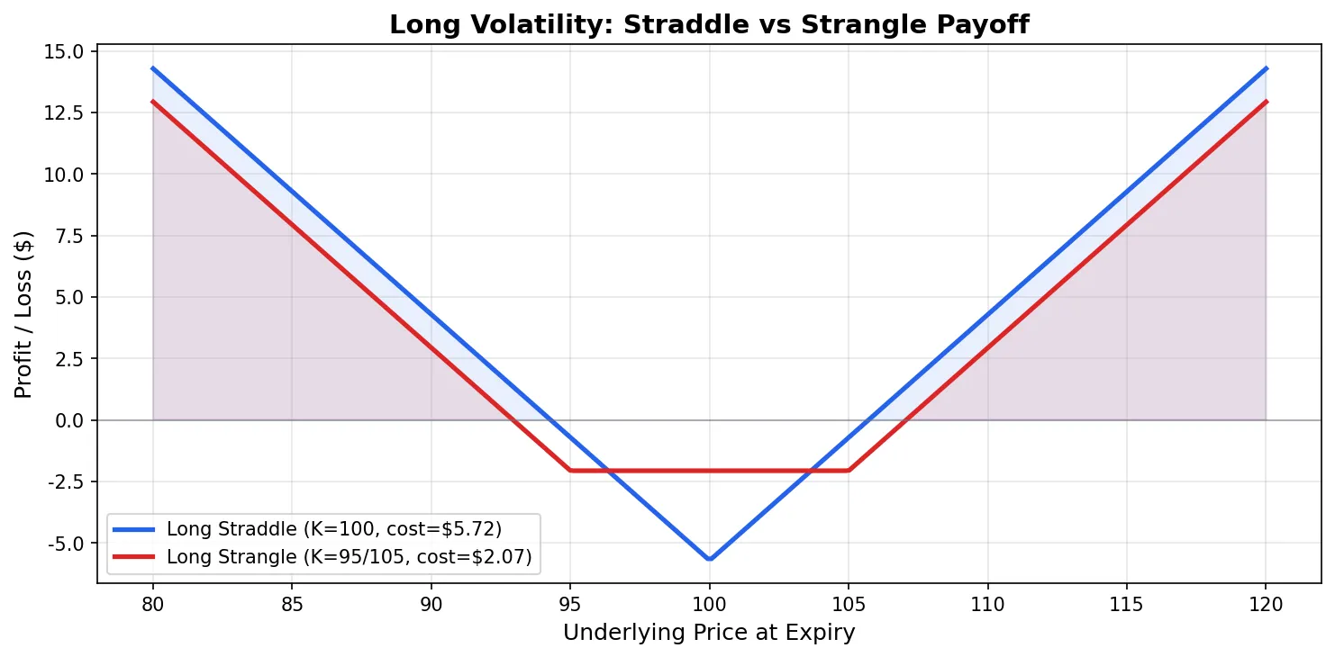
Long Strangle
Construction: buy an OTM call + buy an OTM put. For example, buy the K=105 call + buy the K=95 put.
Both legs are out-of-the-money, so premiums are cheaper. With K=105 call at $1.19 and K=95 put at $0.88, total cost is $2.07.
The tradeoff: breakeven points are further apart ($107.07 up, $92.93 down). The underlying must move more for the trade to profit. If the stock goes from $100 to $103, a straddle might show a small gain, but the strangle is likely still underwater.
When to choose a strangle over a straddle: you expect a large move but want to reduce capital outlay, or your view is that the move will be 8%+ and the strangle’s lower cost gives better leverage on that magnitude.
Calendar Spread (Long Far-Month Vol)
Construction: sell a near-month ATM option + buy a far-month ATM option, same strike.
This strategy goes long vol differently from the previous two. Straddles and strangles bet on an imminent large move. A calendar spread bets that far-month IV will rise (or hold) while near-month time value decays rapidly.
Near-month options lose Theta faster than far-month options. After the near-month leg expires worthless (or is bought back cheaply), the far-month leg retains time value. If IV also rises during this period, the far-month leg benefits from its larger Vega.
The risk: a sudden large move in the near term. If the underlying gaps 10% before the near-month leg expires, the short near-month leg can produce losses exceeding the far-month leg’s gains. Calendar spreads perform best in “quiet now, volatile later” environments.
Another risk is the underlying moving far from the strike. Calendar spreads profit most when the underlying stays near the strike price. A large directional move pushes both legs deep ITM or deep OTM, where time value differences shrink and the trade breaks down.
At near-month expiry, you either close the entire position to lock in profit or loss, or roll the short leg to the next monthly cycle to keep harvesting Theta. Closing only the near-month leg while keeping the far-month leg converts your position from a calendar spread into a naked long option, which has a completely different risk profile.
Three Short Volatility Strategies
Short vol setups fit when IV Rank is elevated and you expect volatility to contract toward normal levels.
Short Straddle
Construction: sell an ATM call + sell an ATM put.
You collect about $5.70 in premium (the mirror image of the long straddle). If the underlying finishes between $94.30 and $105.70 at expiry, you profit. Maximum profit is the $5.70 collected.
Risk is theoretically unlimited. If the underlying drops to $80 or rallies to $120, losses scale with the deviation. Naked short straddles require substantial margin, and most brokers restrict this to accounts with Level 4 or higher options approval.
When to use it: IV Rank above 50%, and you believe the underlying will stay range-bound. The classic setup is post-earnings IV Crush: uncertainty resolves, IV drops from 55% to 30%, and you capture that 25-point Vega gain.
In practice, few traders hold a naked short straddle to expiry. A more common approach is closing the position after IV drops 50%~70%, locking in profits rather than bearing the last few days’ Gamma risk as expiry approaches.
Short Strangle
Construction: sell an OTM call + sell an OTM put. For example, sell the K=105 call + sell the K=95 put.
Compared to a short straddle, the short strangle has a wider profit zone. The underlying can stay anywhere between $95 and $105 without either leg being exercised, providing a thicker cushion. The tradeoff: less premium collected ($2.07 vs. $5.70), lower maximum profit.
Delta selection is the key design choice. Two common approaches:
- 16-Delta Strangle: sell the call and put at Delta ≈ 0.16. Each leg sits roughly one standard deviation from the current price, so each has about a 16% chance of finishing ITM. The probability that neither leg finishes ITM is approximately 68%, and after accounting for collected premium widening the breakeven range, overall probability of profit (POP) is around 72%~75%. Less premium but higher probability of profit.
- 30-Delta Strangle: sell options at Delta ≈ 0.30. Closer to ATM, more premium collected, but a narrower safe zone with a POP of roughly 50%~55%.
The tastytrade-popularized framework of “45 DTE, 16-Delta strangle, enter when collected premium reaches 1% of underlying price” is the most widely adopted short vol starter approach. Whether it works depends on your position sizing and exit discipline, not on the strategy template itself.
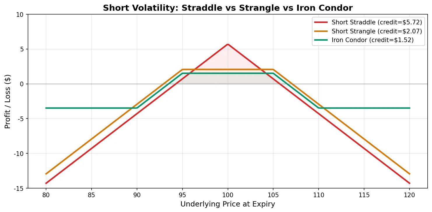
Iron Condor
Construction: short strangle + buy further OTM wings for protection. Specifically: sell K=95 put + buy K=90 put + sell K=105 call + buy K=110 call.
An Iron Condor is a protected short strangle. The purchased wings cap your maximum loss: regardless of how far the underlying moves, the loss is limited to wing width minus net credit received. With $5 wings and $1.50 credit, maximum loss = $5 - $1.50 = $3.50.
Margin requirements drop dramatically. A naked short strangle might require $10,000+ in margin; an Iron Condor needs only $500 (= wing width x 100 shares per contract). This makes short vol accessible to smaller accounts.
When to choose an Iron Condor over a short strangle: your account size cannot support naked selling margin, or you refuse to accept theoretically unlimited downside. The Iron Condor is the most retail-friendly short vol strategy available.
Wing width selection: $5 wings provide stronger protection (smaller max loss) but leave less premium after buying the protective legs. $10 or $15 wings cost less for protection but cap losses at a higher level. A useful heuristic: collected premium should be at least one-third of maximum loss. Below that ratio, the risk-reward is unattractive.
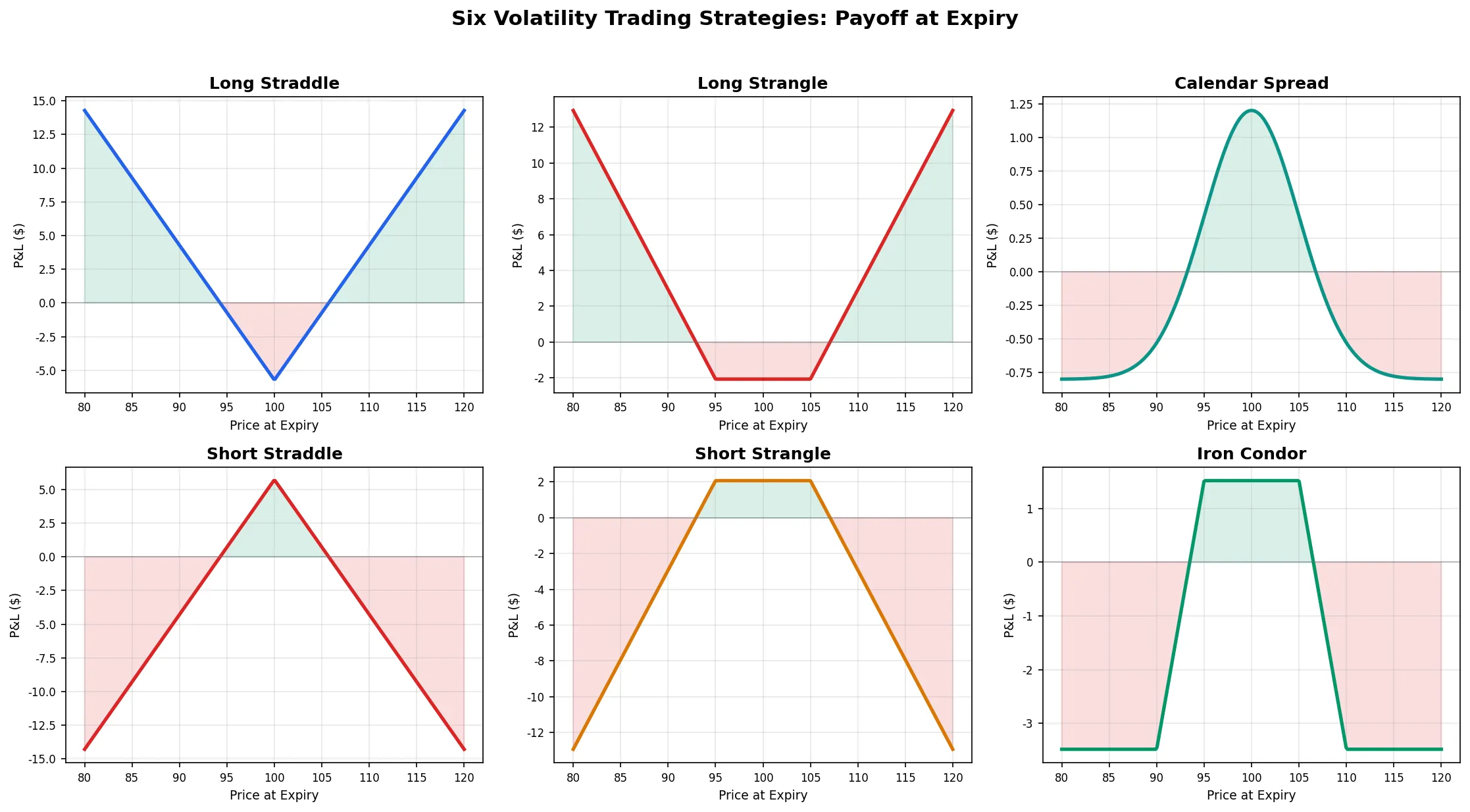
Six Strategies Side by Side
| Strategy | Direction | Max Profit | Max Loss | Vega | Theta | Best IV Environment | Best For |
|---|---|---|---|---|---|---|---|
| Long Straddle | Long vol | Unlimited | Premium paid | + | - | IV low | Expecting a big move, direction unknown |
| Long Strangle | Long vol | Unlimited | Premium paid | + | - | IV low | Lower-cost alternative to straddle |
| Calendar Spread | Long far-month vol | Limited | Net debit | + | + | Near IV high, far IV low | Term structure trades |
| Short Straddle | Short vol | Premium received | Unlimited | - | + | IV high | High-conviction range-bound, large margin |
| Short Strangle | Short vol | Premium received | Unlimited | - | + | IV high | Most popular short vol strategy |
| Iron Condor | Short vol | Net credit | Wing width - credit | - | + | IV high | Retail-friendly, defined risk |
Decision path:
- Check IV Rank and IV Percentile to gauge whether current vol is cheap or rich
- Vol is cheap: go long. Cost-sensitive traders pick the strangle, those wanting maximum Gamma exposure pick the straddle, and term-structure traders pick the calendar spread
- Vol is rich: go short. Large accounts comfortable with unlimited risk use short strangles or short straddles; smaller or risk-averse accounts use Iron Condors
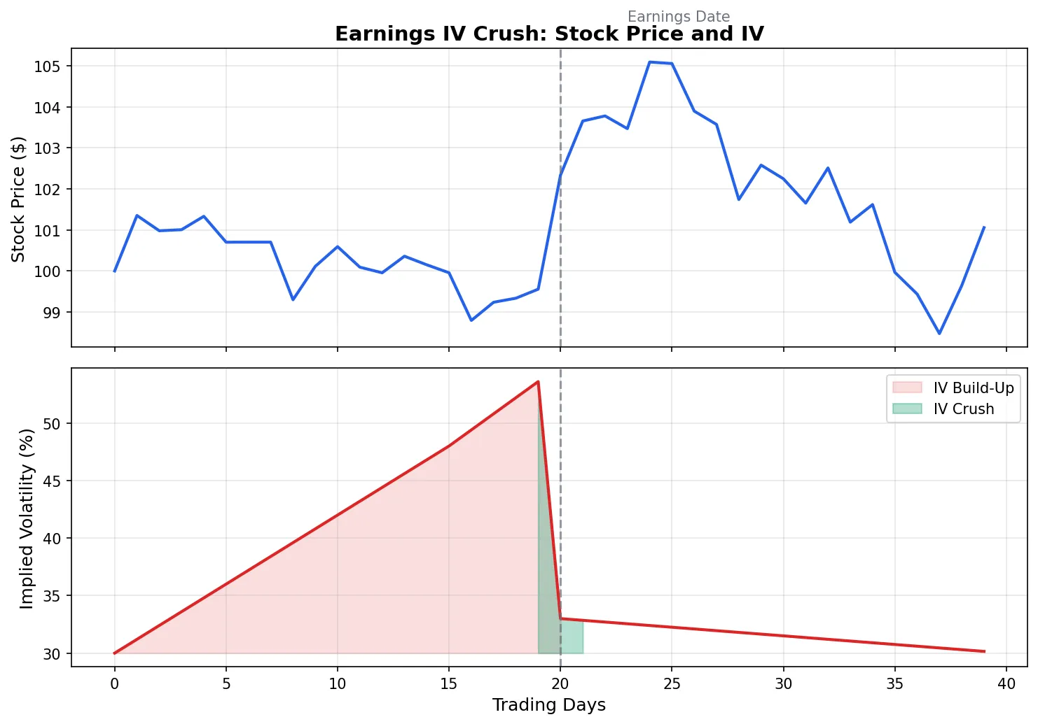
Earnings Volatility Trade: A Worked Example
Earnings announcements are the most concentrated volatility trading opportunity. Pre-earnings uncertainty inflates IV; post-earnings clarity collapses it. This “IV Crush” is nearly universal every earnings season.
A typical scenario: a tech stock’s normal IV is 30%. The week before earnings, IV climbs to 55%. Earnings come out after the close, the stock gaps up 4% next morning, and IV collapses to 32%.
If you sold a 30-Delta short strangle the day before earnings with one week to expiry, you might collect around $3.50 in premium (IV at 55% inflates premiums well above normal). Next morning, IV falls from 55% to 32%, generating roughly $2.80 in Vega profit. The stock’s 4% gap puts your OTM call leg underwater by about $1.20. Net P&L: approximately +$1.60. These numbers are simplified estimates; actual results depend on exact strikes and expiry, but the proportions hold: IV Crush Vega gains exceeded the directional Delta loss.
But had the stock gapped 12% instead of 4%, the call leg loss would have overwhelmed Vega gains, producing a net loss.
Earnings trades are not “IV always drops, so sell straddles for free money.” The market’s Expected Move (the implied straddle-based forecast of the underlying’s move by expiry) prices this balance point precisely. A short strangle profits only when the actual move is smaller than the Expected Move. If your strikes sit inside the Expected Move, your probability of profit is roughly 50%, not the 68% that Delta selection might suggest.
Timing matters. Selling too early (two weeks before earnings) means IV might still be climbing and you take Vega losses before the Crush arrives. Selling too late (the day before) means IV is already peaked but Theta is burning fast and Gamma is enormous, so a small underlying move creates large Delta exposure. Many earnings volatility traders enter 1 to 3 days before the announcement, balancing IV level against Theta/Gamma dynamics.
Common Mistakes and Risk Warnings
“Selling vol is steady income.” Most months it is, just as insurance companies collect premiums most quarters. The problem is tail risk. On February 5, 2018, VIX surged from 17 to 37 in a single session. XIV, the inverse VIX ETN, went to zero overnight. Short vol funds lost several years of accumulated profits in one day. If your position sizing cannot survive a “VIX doubles in one day” scenario, selling vol is Russian roulette with better odds.
“Buy a straddle before earnings and you profit if the stock moves.” This ignores IV Crush. Suppose the stock moves 5% and your call leg gains $4.00 directionally. But IV drops from 55% to 32%, producing $3.20 in Vega losses. Net gain: $0.80, and after two legs’ worth of Theta decay, you might break even or lose. A straddle does not just need the stock to move, it needs the stock to move more than the Expected Move already priced in.
Going long vol when IV is already elevated. If IV Rank exceeds 80%, the straddle you are buying is expensive. Even if the underlying does move, IV is likely to revert lower, and Vega losses eat into your Gamma gains. The best time to go long vol is when IV is low and you have reason to expect it will rise.
Position sizing. For any single short vol trade, maximum potential loss should not exceed 3%~5% of your account. Use Iron Condors instead of naked short strangles, not as a style preference, but as a survival strategy. Ten small wins do not compensate for one catastrophic loss.
Where to Go From Here
These six strategies cover the core volatility trading toolkit. The starting point for strategy selection is gauging IV levels (IV Rank + IV Percentile), then matching to your risk tolerance and account constraints.