This vectorbt tutorial starts from the real difference between vectorized and event-driven backtesting, then walks through the three Portfolio constructors (from_holding, from_signals, from_orders), runs a 10,000-combination grid search, and ends with the freq, signal-shift, and memory traps that quietly produce wrong numbers.
What vectorbt is and why not just use backtrader
vectorbt is a Python backtesting library by Oleg Polakow. The defining difference from backtrader or zipline is the programming model: traditional frameworks march through bars one event at a time and run one strategy instance per loop. vectorbt treats the entire price series and signal series as NumPy matrices, packs many parameter combinations into the column dimension, and computes them all in one pass.
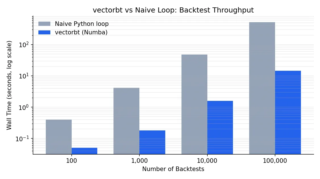
The hot path is JIT-compiled by Numba, with optional Rust kernels (pip install -U "vectorbt[rust]") for the most performance-critical sections. The result: 10,000 dual-SMA backtests on a single core finish in roughly 15 seconds, the same workload in backtrader takes well over an hour.
| Dimension | vectorbt | backtrader | zipline |
|---|---|---|---|
| Programming model | Vectorized matrix ops | Event-driven, bar by bar | Event-driven |
| Parameter sweeps | Native, single pass | Outer loop required | Outer loop required |
| Speed | Very fast (Numba/Rust) | Moderate (pure Python) | Moderate |
| Learning curve | Needs pandas multi-index fluency | OOP-friendly | Similar to backtrader |
| Complex order logic | Awkward | First-class | First-class |
| Best at | Factor research, parameter sweeps | Strategy prototyping, live trading | Quantopian compatibility |
When vectorbt is the wrong choice: strategies with strong path dependence such as trade-state-based pyramiding, multi-leg option hedges, or order chains where bar t+1 depends on the fill of bar t. Expressing those as vectors gets ugly fast, and backtrader’s event loop is the cleaner tool. vectorbt’s sweet spot is the research phase: when the question is “what if I changed the window, the asset, the stop level” and you want all answers at once.
Install and your first backtest in five lines
Minimal install:
pip install -U vectorbt
With the Rust engine or TA-Lib integration:
pip install -U "vectorbt[rust]"        # Rust acceleration
pip install -U "vectorbt[full]"        # TA-Lib, Pandas TA, etc.
pip install -U "vectorbt[full,rust]"   # everything
A buy-and-hold backtest on Bitcoin in five lines:
import vectorbt as vbt

data = vbt.YFData.download("BTC-USD")
price = data.get("Close")

pf = vbt.Portfolio.from_holding(price, init_cash=100)
print(pf.total_profit())
vbt.YFData is a thin wrapper over yfinance that returns a Data object; .get("Close") pulls a one-column close-price Series. Portfolio.from_holding is the simplest constructor: it goes all-in on the first bar, holds, and exits on the last bar.
The price here is one-dimensional (single asset, single config). vectorbt’s real power kicks in once price becomes a 2D DataFrame whose columns represent different assets or different parameter combinations. Every operation broadcasts across columns automatically. Holding that mental model is the prerequisite for the parameter-sweep section below.
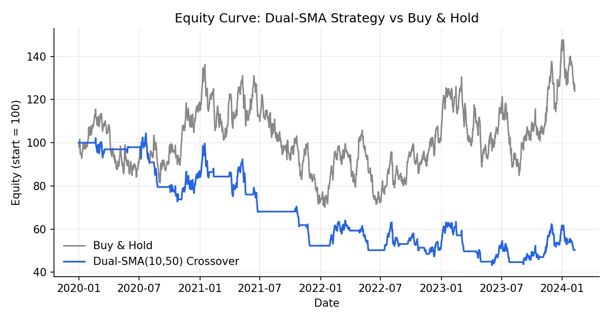
Dual-SMA crossover: from signal to portfolio
The textbook trend-following setup: enter when the fast SMA crosses above the slow SMA, exit on the opposite cross.
fast_ma = vbt.MA.run(price, 10)
slow_ma = vbt.MA.run(price, 50)

entries = fast_ma.ma_crossed_above(slow_ma)
exits = fast_ma.ma_crossed_below(slow_ma)

pf = vbt.Portfolio.from_signals(
    price, entries, exits,
    init_cash=100,
    fees=0.001,        # 10 bps per side
    slippage=0.001,    # 10 bps slippage
    freq="1D",         # daily bars; required for annualized metrics
)
print(pf.stats())
vbt.MA.run returns an Indicator instance, not a plain Series. It carries the raw MA values plus a family of comparison helpers (ma_crossed_above, ma_crossed_below, ma_above). entries and exits are boolean Series where True marks the bar that triggers a buy or sell.
Portfolio.from_signals translates signals into a portfolio: at every entries=True bar it buys with all available cash, at every exits=True bar it closes the position. stats() produces a performance table:
Start                          2017-11-09
End                            2026-01-03
Total Return [%]               1504.09
Benchmark Return [%]            866.09
Max Drawdown [%]                 70.73
Total Trades                       81
Win Rate [%]                    41.25
Sharpe Ratio                     0.86
Sortino Ratio                    1.30
Calmar Ratio                     0.57
A 41% win rate but nearly 2x the buy-and-hold return is the classic trend-follower fingerprint: most signals lose, the winners pay for them.
A few stats fields that newcomers tend to skip past: Calmar Ratio (annualized return over max drawdown) is more honest than Sharpe for trend strategies. Profit Factor (gross wins over gross losses) needs to clear roughly 1.5 to suggest a real edge. The gap between Avg Winning Trade Duration and Avg Losing Trade Duration measures how well the strategy lets winners run and cuts losers short.
Choosing among from_holding, from_signals, from_orders
vectorbt’s Portfolio exposes three primary factory methods, and confusion about which one to use is the single most common beginner stumbling block.
| Constructor | Inputs | Semantics | Typical use |
|---|---|---|---|
from_holding | Price | Buy on bar 0, hold to the end | Benchmarks, long-term DCA |
from_signals | Price + entries/exits booleans | Buy on True entries, sell on True exits, default size = max | Trend following, indicator strategies |
from_orders | Price + per-bar order size | Specify how many units to buy/sell each bar | Rebalancing, momentum weighting |
Together they cover roughly 95% of backtesting workflows. from_signals is the workhorse, but it has one default that quietly burns people: consecutive entries=True bars after the first one are ignored because the position is already on. If your strategy pyramids, you must pass accumulate=True explicitly. The same goes for exits: they only do anything when there is a position to close.
from_orders gives you the most control:
import numpy as np
import pandas as pd

orders = pd.Series(0.0, index=price.index)
orders.iloc[0] = 1.0     # buy 1 unit on bar 0
orders.iloc[100] = -1.0  # sell 1 unit on bar 100

pf = vbt.Portfolio.from_orders(price, orders, init_cash=100, freq="1D")
Positive size buys, negative sells, zero is a no-op. Monthly rebalancing, vol-weighted sizing, risk parity all live here.
The point of vectorization: 10,000 backtests in one pass
This is where vectorbt earns its name. Take the dual-SMA strategy and grid-search every fast/slow window pair. In a traditional framework that means two nested loops and a long coffee break. In vectorbt it is a few lines and roughly 15 seconds.
import numpy as np

symbols = ["BTC-USD", "ETH-USD", "XRP-USD"]
data = vbt.YFData.download(symbols, missing_index="drop")
price = data.get("Close")

windows = np.arange(2, 101)
fast_ma, slow_ma = vbt.MA.run_combs(
    price, window=windows, r=2, short_names=["fast", "slow"]
)
entries = fast_ma.ma_crossed_above(slow_ma)
exits = fast_ma.ma_crossed_below(slow_ma)

pf = vbt.Portfolio.from_signals(
    price, entries, exits,
    size=np.inf, fees=0.001, freq="1D",
)
vbt.MA.run_combs(window=windows, r=2) is the load-bearing call: it picks 2-element combinations from windows (C(99, 2) ≈ 4,851 pairs) and produces matched fast/slow MA columns. Multiplied by 3 symbols, entries becomes a DataFrame with over 14,000 columns. Portfolio swallows it whole and backtests every column independently.
For visualization, vectorbt ships a heatmap accessor:
fig = pf.total_return().vbt.heatmap(
    x_level="fast_window",
    y_level="slow_window",
    slider_level="symbol",
    symmetric=True,
    trace_kwargs=dict(colorbar=dict(title="Total return", tickformat="%")),
)
fig.show()
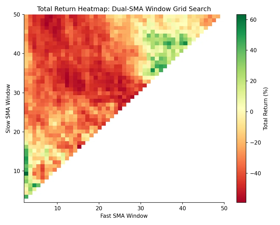
The heatmap shows which parameter regions are stably profitable versus which are isolated peaks (a textbook overfitting tell). A broad plateau is far more trustworthy than a sharp single-cell maximum. Parameter-stability analysis at this granularity is standard factor-research practice, and impractical without vectorbt-class speed.
Drill into a specific configuration:
print(pf[(10, 20, "ETH-USD")].stats())
pf[(10, 20, "ETH-USD")].plot().show()
pf[(fast, slow, symbol)] is pandas multi-index slicing. The selected column behaves like a single-strategy portfolio, with the same stats and plot APIs.
Why vectorbt is fast: Numba plus structured NumPy
A naive Python loop running 10,000 backtests takes around 8 minutes. vectorbt does the same workload in roughly 15 seconds. Three reasons.
First, every strategy instance lives as a column in a single 2D NumPy array. pandas DataFrames align column-wise for free, so a comparison like fast_ma > slow_ma runs across all columns in one C-level call, with no Python-side loop.
Second, the hot paths are decorated with Numba’s @njit. The Python bytecode is compiled to machine code on first call and runs at near-C speed thereafter. The most performance-critical kernels (order matching, portfolio-state updates) also have optional Rust implementations, automatically used once vectorbt[rust] is installed.
Third, no per-event objects. backtrader allocates a Bar object per bar and an Order object per order; allocation and GC pressure dominate. vectorbt operates on flat structured NumPy arrays end to end, with zero per-event allocation.
The exact numbers vary with strategy complexity, data size, and hardware. The order of magnitude does not.
Pitfalls and best practices
This section is what the docs underweight, and every item below directly determines whether your backtest numbers are real.
Always set freq explicitly. Without it, annualized return, Sharpe, and Sortino are all wrong. vectorbt falls back to a guess based on bar count divided by 252 or 365, but your bars might be 5-minute, hourly, or weekly. Every time-normalized metric depends on freq to convert correctly.
To shift signals or not. The textbook lookahead trap. fast_ma.ma_crossed_above(slow_ma) computes its signal at bar t using bar t’s close, so the signal already incorporates the close-bar information. Portfolio.from_signals defaults to filling on the same bar at price (which defaults to close), which means you are effectively buying at the same close that produced the signal — fine in backtest, impossible in live trading. The clean fixes are either to shift(1) your entries and exits, or to pass next-bar open prices explicitly: Portfolio.from_signals(open_price, entries.shift(1), ...). See backtesting pitfalls for the broader catalog of lookahead traps.
Multi-asset alignment. vbt.YFData.download(symbols) defaults to a union of timestamps with NaN fill. That lets one asset participate in computations during periods when it had not yet started trading, which corrupts results. The right default is missing_index="drop", keeping only timestamps where every asset has data.
Memory blowups. A 10,000-column backtest stores trades and drawdowns per column. Multiply by several assets and a long history and you can fill 30 GB of RAM in a few minutes. The most reliable workaround is a manual column-batch loop that extracts only the metrics you need before discarding each chunk:
chunk = 500
results = []
for i in range(0, entries.shape[1], chunk):
    sub_pf = vbt.Portfolio.from_signals(
        price, entries.iloc[:, i:i+chunk], exits.iloc[:, i:i+chunk],
        size=np.inf, fees=0.001, freq="1D",
    )
    # Keep only the lightweight metric you actually need
    results.append(sub_pf.total_return())
total_return = pd.concat(results)
Each iteration’s Portfolio object is GC’d before the next chunk runs, so peak memory drops from full × N to chunk size. vectorbt also exposes a chunked decorator module for more automated patterns; the PRO edition adds Portfolio-aware merge functions on top of that.
Local data as a fallback. When yfinance is unreliable (rate limits, regional blocks), local CSVs are the simplest substitute:
import pandas as pd
df = pd.read_csv("btc.csv", index_col="date", parse_dates=True)
price = df["close"]
# feed straight into from_signals
Anything that lands in a Series or DataFrame with a DatetimeIndex works. The downstream API does not care where the data came from.
Where to go next: community vs PRO
vectorbt has a free community edition (used throughout this article) and a commercial PRO edition. The community version already covers single-asset prototyping, parameter sweeps, and factor research. PRO unlocks four families of features: granular order types (limit, stop-loss, take-profit), built-in portfolio optimization and risk parity, parallel execution, and research tools like pattern recognition and event projections.
The fastest learning path: read the official Usage page end to end, then work through the example notebooks, focusing on the dual-SMA sweep, Bollinger Bands, and portfolio-level trade analysis. Those three cover roughly 80% of common patterns. When you get stuck, read the source. The author’s docstrings are dense and almost always faster than searching Stack Overflow.
The moment your first parameter sweep finishes in seconds rather than hours is the moment “vectorization” stops being a buzzword. Research cadence changes, and so do the questions you can afford to ask.