Quant trading articles are full of math terms: log returns, standard deviation, covariance matrices, OLS regression, partial derivatives. You can look up each definition, but without the trading context, the definitions don’t stick. This article goes through the most common math concepts in quant trading, each anchored to a real trading scenario with Python code.
Log Returns
A stock goes from $100 to $110. What’s the return?
The intuitive answer is the simple return: \((110 - 100) / 100 = 10\%\). But quant finance uses log returns: \(\ln(110 / 100) = 9.53\%\).
The formulas:
$$ R_{\text{simple}} = \frac{P_t - P_{t-1}}{P_{t-1}} = \frac{P_t}{P_{t-1}} - 1 $$$$ R_{\text{log}} = \ln\left(\frac{P_t}{P_{t-1}}\right) $$Why does quant finance prefer log returns? Three reasons.
Additivity. Simple returns don’t add up correctly. A stock that goes up 10% then down 10% has simple returns summing to 0%, but you actually lost 1% (100 → 110 → 99). Log returns add correctly: the sum of multi-period log returns equals the log return over the entire period. This saves a lot of headache when computing cumulative returns or rolling window metrics.
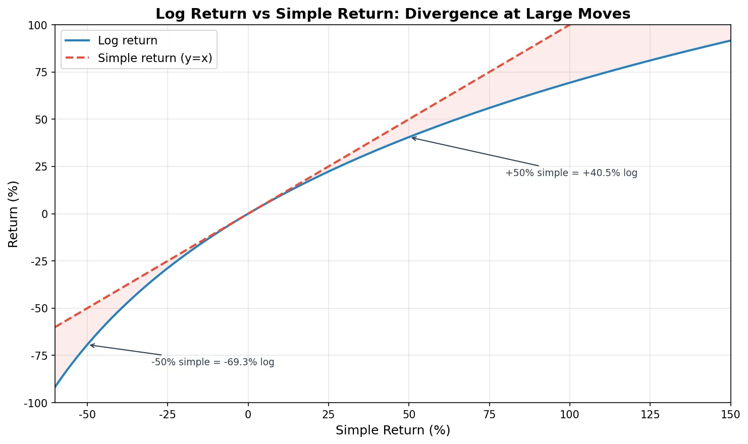
Symmetry. With simple returns, a 50% gain (100→150) and a 33.3% loss (150→100) are the “reverse” of each other, but the numbers are asymmetric. Log returns give +40.5% and -40.5%, perfectly symmetric.
Approximation. For small moves (daily returns within ±2%), the two are nearly identical (difference under 0.02 percentage points). So for everyday use there’s no practical difference, but log returns are mathematically much cleaner.
import numpy as np

prices = np.array([100, 110, 104.5, 120, 96])
simple_ret = np.diff(prices) / prices[:-1]
log_ret = np.log(prices[1:] / prices[:-1])

for i in range(len(simple_ret)):
    print(f"Day {i+1}: simple={simple_ret[i]*100:+.2f}%  "
          f"log={log_ret[i]*100:+.2f}%")

print(f"\nSum of simple returns: {simple_ret.sum()*100:.2f}%")
print(f"Sum of log returns:    {log_ret.sum()*100:.2f}%")
print(f"Actual total return:   {(prices[-1]/prices[0]-1)*100:.2f}%")
print(f"exp(sum of log ret):   {(np.exp(log_ret.sum())-1)*100:.2f}%")
Day 1: simple=+10.00%  log=+9.53%
Day 2: simple=-5.00%   log=-5.13%
Day 3: simple=+14.83%  log=+13.83%
Day 4: simple=-20.00%  log=-22.31%

Sum of simple returns: -0.17%
Sum of log returns:    -4.08%
Actual total return:   -4.00%
exp(sum of log ret):   -4.00%
Simple returns sum to -0.17%, but the stock actually fell 4%. Log returns sum to -4.08%, and converting back (exp) gives exactly -4.00%. That’s additivity in action.
The larger the price move, the bigger the gap. Day 4 dropped 20% in simple terms but -22.31% in log terms, a 2.31 percentage point difference. In crypto markets where 10%+ daily moves are routine, this gap matters even more.
Mean, Variance, and Standard Deviation
Mean measures “how much do you earn on average.” Standard deviation measures “how stable are those earnings.” In quant trading, return and risk are defined by these two numbers.
The formulas:
$$ \mu = \frac{1}{n}\sum_{i=1}^{n} r_i, \quad \sigma = \sqrt{\frac{1}{n-1}\sum_{i=1}^{n}(r_i - \mu)^2} $$The Sharpe Ratio is the most classic combination of mean and standard deviation:
$$ \text{Sharpe} = \frac{\mu - R_f}{\sigma} $$The numerator is excess return (above the risk-free rate), the denominator is volatility. The intuition: “for each unit of risk, how much excess return did you earn?” A Sharpe of 1.0 is decent, above 2.0 is excellent, below 0.5 means the volatility isn’t worth it.
Annualization is a detail that trips people up. Multiply daily mean return by 252 (trading days) for annualized return. Multiply daily standard deviation by \(\sqrt{252}\) for annualized volatility. Why the square root for standard deviation? Because the variance of independent random variables is additive (\(\text{Var}(X_1 + X_2) = \text{Var}(X_1) + \text{Var}(X_2)\)), so 252-day variance = daily variance × 252, and standard deviation = \(\sqrt{252}\) × daily std.
import numpy as np

np.random.seed(42)
daily_returns = np.random.normal(0.0004, 0.015, 252)

mean_daily = daily_returns.mean()
std_daily = daily_returns.std(ddof=1)  # ddof=1: sample std
rf_daily = 0.04 / 252  # 4% annual risk-free rate

sharpe = (mean_daily - rf_daily) / std_daily * np.sqrt(252)
annual_return = mean_daily * 252
annual_vol = std_daily * np.sqrt(252)

print(f"Annual return:     {annual_return*100:.2f}%")
print(f"Annual volatility: {annual_vol*100:.2f}%")
print(f"Sharpe ratio:      {sharpe:.2f}")
Annual return:     8.66%
Annual volatility: 23.03%
Sharpe ratio:      0.20
8.66% annual return with 23.03% volatility gives a Sharpe of only 0.20. The return is almost entirely eaten by the volatility. Risk-adjusted, this is a poor result.
Normal Distribution and Fat Tails
The Normal Distribution is the most common assumption in quant finance. Its probability density function:
$$ f(x) = \frac{1}{\sigma\sqrt{2\pi}} \exp\left(-\frac{(x-\mu)^2}{2\sigma^2}\right) $$The useful rule of thumb: 68% of data falls within \(\mu \pm 1\sigma\), 95% within \(\mu \pm 2\sigma\), 99.7% within \(\mu \pm 3\sigma\). Under a normal distribution, events beyond 3σ have a probability of only 0.3%, roughly once a year.
The problem: stock returns are not truly normal.
Real return distributions have thicker tails than the normal distribution, a property called fat tails (or leptokurtosis). Extreme events beyond 3σ happen far more often than the normal distribution predicts. A simulation comparison: the normal distribution predicts about 14 events beyond 3σ in 5,000 trading days, but a fat-tailed distribution produces 60-80 such events, 4-5 times more.
This directly affects risk management. VaR (Value at Risk) is one of the most common risk metrics, and many VaR calculations assume normally distributed returns. If the actual distribution has fat tails, normal VaR severely underestimates the probability of extreme losses. During the 2008 financial crisis, many quant funds blew up partly because their models assumed normality while markets delivered 6σ or even 10σ events that were “impossible” under their models. The March 2020 crash was a more recent reminder: the S&P 500 hit multiple daily moves beyond 4σ within a single week.
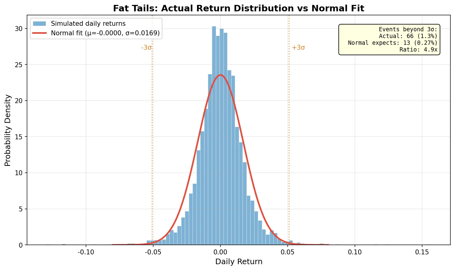
The blue histogram shows simulated returns with fat-tail characteristics. The red line is a normal distribution fitted with the same mean and standard deviation. The tails clearly extend beyond what the normal curve predicts.
Covariance and Correlation
For a single stock, mean and standard deviation are enough. With two or more stocks in a portfolio, you need covariance to describe how they relate.
$$ \text{Cov}(A, B) = \frac{1}{n-1}\sum_{i=1}^{n}(A_i - \bar{A})(B_i - \bar{B}) $$Positive covariance means the two stocks tend to move together; negative means they tend to move in opposite directions. But the raw number is hard to interpret (it depends on the scale of returns), so we standardize it into correlation:
$$ \rho_{A,B} = \frac{\text{Cov}(A, B)}{\sigma_A \cdot \sigma_B}, \quad \rho \in [-1, 1] $$\(\rho = 1\) means perfect positive correlation, \(\rho = -1\) perfect negative, \(\rho = 0\) no linear relationship.
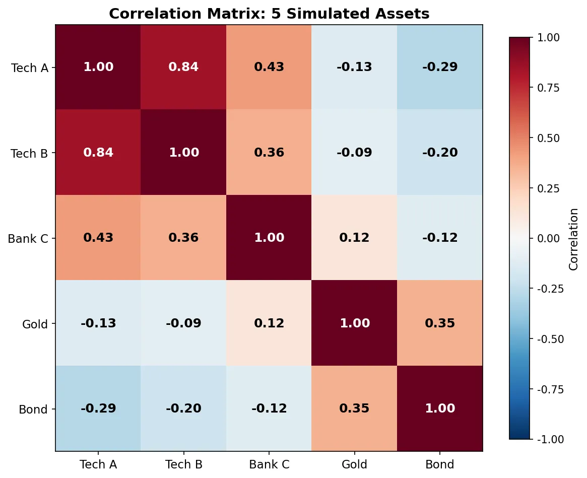
Arrange all pairwise covariances of N assets into an \(N \times N\) matrix and you get the covariance matrix \(\Sigma\). This matrix appears constantly in quant trading: pairs trading uses correlation to find co-moving stocks, portfolio optimization uses the covariance matrix to minimize risk, factor models use covariance structure to analyze factor relationships.
Portfolio variance is easier to understand with a concrete two-asset example. Suppose you hold 60% in stock A (20% annual vol) and 40% in stock B (15% annual vol), with correlation 0.3:
$$ \sigma_p^2 = 0.6^2 \times 0.20^2 + 0.4^2 \times 0.15^2 + 2 \times 0.6 \times 0.4 \times 0.20 \times 0.15 \times 0.3 = 0.02232 $$Portfolio volatility: \(\sigma_p = \sqrt{0.02232} = 14.94\%\). If the two were perfectly correlated (\(\rho = 1\)), portfolio vol would be 18% (a weighted average). A correlation of 0.3 brings it down from 18% to 14.94%. That’s the math behind diversification. One catch: correlations look stable during calm markets but spike toward 1.0 in a crash. During the March 2020 meltdown, stocks, commodities, and credit all moved in lockstep. Diversification failed precisely when it was needed most. Keep this in mind when building portfolios from historical correlation data.
For N assets, the formula generalizes to matrix notation:
$$ \sigma_p^2 = \mathbf{w}^T \Sigma \mathbf{w} $$where \(\mathbf{w}\) is the weight vector and \(\Sigma\) is the covariance matrix.
import numpy as np

np.random.seed(2024)
n = 252

stock_a = np.random.normal(0.0005, 0.02, n)
stock_b = 0.6 * stock_a + np.random.normal(0.0002, 0.015, n)
stock_c = -0.3 * stock_a + np.random.normal(0.0003, 0.018, n)

returns = np.column_stack([stock_a, stock_b, stock_c])
cov_matrix = np.cov(returns.T)
corr_matrix = np.corrcoef(returns.T)

labels = ['Stock A', 'Stock B', 'Stock C']
print("=== Correlation Matrix ===")
for i, label in enumerate(labels):
    row = '  '.join(f'{corr_matrix[i,j]:+.4f}' for j in range(3))
    print(f"  {label}: {row}")
=== Correlation Matrix ===
  Stock A: +1.0000  +0.5393  -0.4396
  Stock B: +0.5393  +1.0000  -0.1537
  Stock C: -0.4396  -0.1537  +1.0000
Stock A and B have correlation +0.54 (moderate positive, tend to move together). A and C have correlation -0.44 (negative, tend to move opposite). A portfolio of only A and B gets limited diversification benefit; adding C with its negative correlation substantially reduces portfolio volatility.
Linear Regression (OLS)
OLS (Ordinary Least Squares) is the most widely used statistical tool in quant trading. The idea is simple: given a set of data points, find the line that minimizes the sum of squared residuals (distances from each point to the line).
For \(y = \alpha + \beta x + \varepsilon\), the OLS solution is:
$$ \hat{\beta} = \frac{\sum(x_i - \bar{x})(y_i - \bar{y})}{\sum(x_i - \bar{x})^2} $$In matrix form for multiple variables:
$$ \hat{\boldsymbol{\beta}} = (\mathbf{X}^T \mathbf{X})^{-1} \mathbf{X}^T \mathbf{y} $$OLS shows up in two key quant trading contexts:
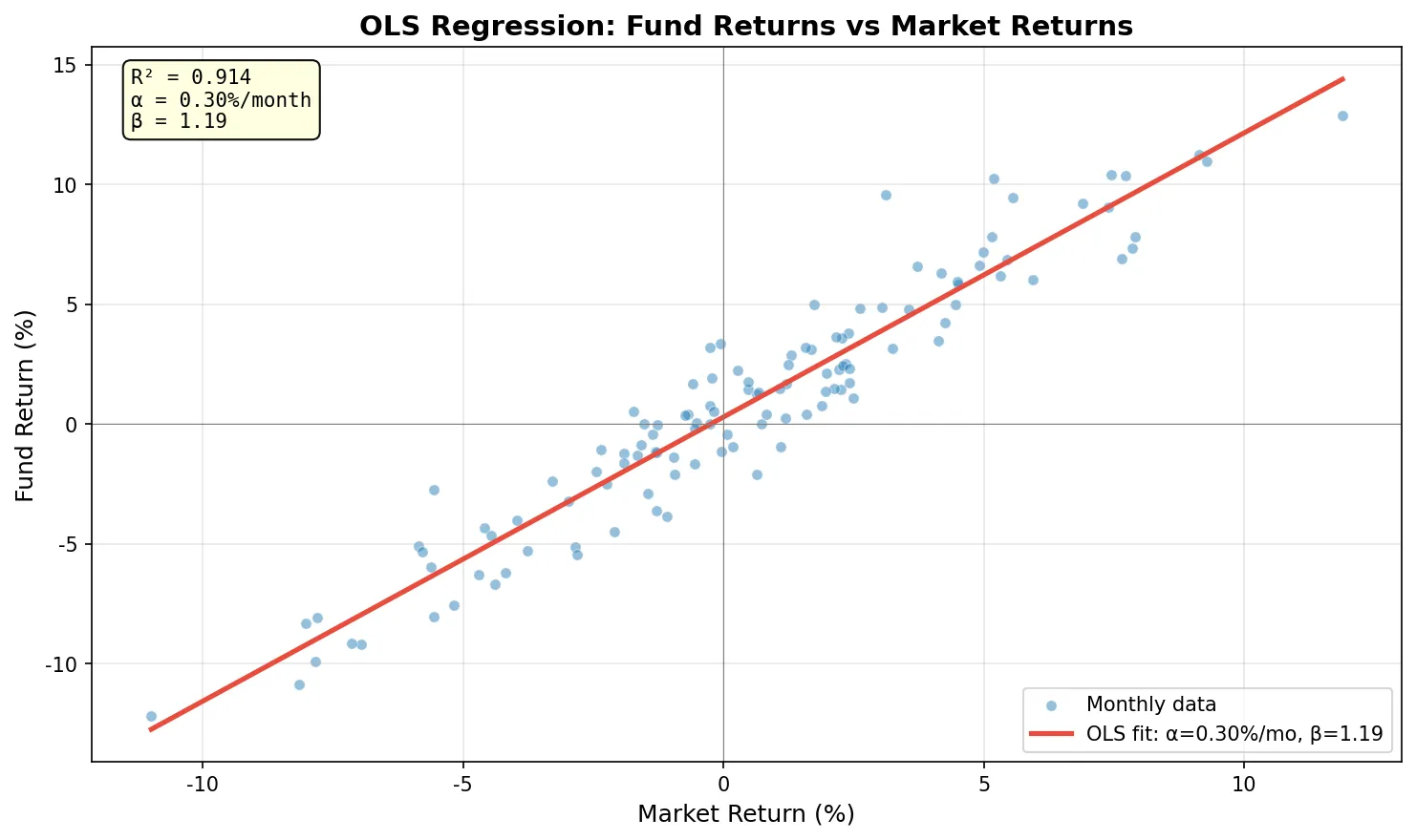
Factor regression. The Fama-French factor model uses OLS to decompose fund returns into contributions from market, size, value, and other factors. The regression’s \(\alpha\) represents excess return that factors can’t explain; \(\beta\) coefficients measure factor exposures.
Pairs trading. Two correlated stocks A and B are regressed as \(A = \alpha + \beta B + \varepsilon\). The residual \(\varepsilon\) is the spread. When the spread deviates far from its mean, you trade mean reversion.
import numpy as np

np.random.seed(42)
n = 120  # 10 years monthly
market = np.random.normal(0.008, 0.045, n)
fund = 0.002 + 1.15 * market + np.random.normal(0, 0.015, n)

X = np.column_stack([np.ones(n), market])
beta, _, _, _ = np.linalg.lstsq(X, fund, rcond=None)

pred = X @ beta
ss_res = np.sum((fund - pred) ** 2)
ss_tot = np.sum((fund - fund.mean()) ** 2)
r2 = 1 - ss_res / ss_tot

mse = ss_res / (n - 2)
se = np.sqrt(np.diag(mse * np.linalg.inv(X.T @ X)))
t_stats = beta / se

print(f"Alpha: {beta[0]*100:.3f}% /month  (t={t_stats[0]:.2f})")
print(f"Beta:  {beta[1]:.3f}           (t={t_stats[1]:.2f})")
print(f"R²:    {r2:.4f}")
Alpha: 0.296% /month  (t=2.12)
Beta:  1.186           (t=35.50)
R²:    0.9144
Beta of 1.186 means the fund swings more than the market (market up 1%, fund up ~1.19% on average). Alpha of 0.296%/month with t=2.12 is marginally significant at the 5% level, suggesting some excess return but not with high confidence. R² of 0.91 means the market factor explains 91% of the fund’s return variation.
Two common pitfalls. High R² doesn’t mean good predictions. R² = 0.91 only means the past fit is good; it guarantees nothing about the future. Overfitted models routinely show R² near 1.0 in-sample and collapse out-of-sample. Correlation is not causation. Two stocks being highly correlated might just mean they share the same industry factor. Using one to predict the other without understanding the underlying mechanism is risky.
Derivatives and Partial Derivatives
A derivative measures the rate of change of a function. \(f'(x)\) tells you “if x changes a tiny bit, how much does f(x) change?”
Option prices depend on multiple variables: underlying price \(S\), time to expiry \(t\), volatility \(\sigma\), interest rate \(r\). A partial derivative holds all other variables fixed and measures the effect of changing just one.
The Greeks that option traders watch every day are partial derivatives:
$$ \Delta = \frac{\partial V}{\partial S}, \quad \Theta = \frac{\partial V}{\partial t}, \quad \text{Vega} = \frac{\partial V}{\partial \sigma} $$\(\Delta = 0.6\) means: if the underlying rises by $1, the option price rises by roughly $0.60. \(\Theta = -0.05\) means: each passing day costs the option roughly $0.05 in time decay. Vega = 0.15 means: if implied volatility rises by 1 percentage point, the option price rises by roughly $0.15.
You don’t need to derive Black-Scholes from scratch to understand Greeks. The core intuition is one sentence: Greeks quantify how sensitive the option price is to each input variable. Traders use Delta to decide how many shares to hedge, Theta to evaluate time decay costs, and Vega to assess volatility risk. For detailed Greeks calculations and applications, see the Option Greeks series.
If you want to verify computationally, the simplest method is finite difference: nudge the underlying price by a small amount (say $0.01), compute the option price twice, and divide the difference by the step size. This is exactly the definition of a partial derivative: \(\frac{\partial V}{\partial S} \approx \frac{V(S+h) - V(S-h)}{2h}\).
Math Concepts Quick Reference
| Concept | One-line explanation | Quant trading application |
|---|---|---|
| Log return | \(\ln(P_t/P_{t-1})\), additive across periods | Cumulative return calculation, return modeling |
| Mean | Average return | Strategy expected return |
| Standard deviation | Dispersion of returns | Volatility, risk measurement |
| Sharpe ratio | Excess return / std dev | Risk-adjusted strategy performance |
| Normal distribution | Bell curve distribution | VaR calculation, risk modeling |
| Fat tails | Extreme events more frequent than normal | Tail risk management |
| Covariance | Direction and strength of co-movement | Pairs trading, portfolio optimization |
| Correlation | Standardized covariance, [-1, 1] | Finding hedges and co-moving pairs |
| Covariance matrix | N×N matrix of asset relationships | Portfolio risk calculation |
| OLS regression | Line fit minimizing squared residuals | Factor regression, pairs trading spread |
| R² | Proportion of variance explained | Model fit assessment |
| Partial derivative | Rate of change holding other vars fixed | Option Greeks |
Probability and statistics handle “what are this strategy’s returns and risks.” Linear regression answers “where do the returns come from.” Partial derivatives tell you “what happens when a parameter changes.” You don’t need to retake a university math course for quant trading. Get comfortable with the concepts in this table, and the formulas in quant articles will stop being opaque.