Qlib is Microsoft’s open-source AI quant platform, released in 2020 and now sitting at 16k+ stars on GitHub. It bundles data, factors, models, backtesting, and reporting into one pipeline, ships with the Alpha158 and Alpha360 factor sets, and includes 20+ models out of the box (LightGBM, Transformer, TCN, and more). This Qlib tutorial walks from installation to a working LightGBM + Alpha158 strategy, then to reading the backtest report, and ends with a checklist of pitfalls.
By the end you will: have Qlib running locally, have downloaded A-share daily data, train a model in 30 lines, run the standardised qrun workflow, and understand IC, annualised return, and max drawdown numbers in the output.
What Qlib Is and When to Use It
Qlib bills itself as an “AI-oriented quantitative investment platform”. Two keywords there: AI, and quant. It is not a trading engine (unlike vnpy, which connects directly to broker APIs), and not just a backtester (unlike Backtrader, which only cares about strategy logic). Qlib assumes your workflow looks like this: pull historical data, compute factors, train a model, score and rank instruments, build a portfolio from the ranking, backtest, read the report. Every step ships with a working implementation.
Here is how it compares to other common frameworks, based on hands-on use:
| Framework | Strengths | Weaknesses | Typical user |
|---|---|---|---|
| Qlib | End-to-end pipeline (factors + ML + backtest), good A-share data | Steep learning curve, many abstraction layers | Quant researchers doing factor work |
| Backtrader | Flexible, clean event-driven backtests | No data, no factor library, build your own | Strategy developers, CTA traders |
| vnpy | Excellent live trading, full UI | Trading-system focus, weak research tools | China-domestic prop shops |
| Zipline | Classic, well documented | Unmaintained, locked to old pandas | Legacy projects |
| QuantConnect/LEAN | Cloud one-stop shop, multi-market | Closed cloud service, painful local setup | Overseas retail, small teams |
When Qlib is the wrong tool: if you only want a simple two-MA-crossover strategy with no ML, Qlib is overkill; if you do high-frequency or intraday tick work, the 1-min support exists but is not the main use case; if you need live order routing, Qlib does not handle execution and you have to bolt that on yourself.
Installing Qlib and Downloading Data
The fastest path is pip:
pip install pyqlib
Stick to Python 3.8 to 3.11. On Python 3.12 I have seen lightgbm builds fail intermittently on Windows, and on 3.8 some recent pytorch wheels are missing. 3.10 is the sweet spot.
Source install is for people who plan to modify Qlib internals:
git clone https://github.com/microsoft/qlib.git
cd qlib
pip install numpy cython
pip install -e .
The official README still says python setup.py install, but setuptools 58+ deprecated that command and you will get error: invalid command 'install'. Use pip install -e . instead; it works, and editable mode lets you hack on Qlib internals without reinstalling.
One-liner to verify:
import qlib
print(qlib.__version__)  # 0.9.x
Now data. Qlib stores OHLCV in its own columnar .bin format (faster than CSV or parquet), pulled via:
# A-share daily
python -m qlib.run.get_data qlib_data \
    --target_dir ~/.qlib/qlib_data/cn_data \
    --region cn

# US daily
python -m qlib.run.get_data qlib_data \
    --target_dir ~/.qlib/qlib_data/us_data \
    --region us
The full A-share archive is around 2 GB. Connections to the source server are flaky from China; pass --interval 1d explicitly so a retry resumes cleanly. Once done you get:
~/.qlib/qlib_data/cn_data/
├── calendars/        # trading calendar
├── instruments/      # universe definitions (all.txt, csi300.txt, csi500.txt)
├── features/         # one folder per stock, .bin column files inside
└── dataset_cache/
Windows gotcha: ~ does not expand in some shells. Use absolute paths like D:/qlib_data/cn_data everywhere, otherwise Qlib will throw FileNotFoundError and you will spend an hour wondering why.
Train Your First LightGBM Model in 30 Lines
The minimal end-to-end example for any Qlib tutorial, init through prediction:
import qlib
from qlib.constant import REG_CN
from qlib.contrib.data.handler import Alpha158
from qlib.contrib.model.gbdt import LGBModel
from qlib.data.dataset import DatasetH

qlib.init(provider_uri="~/.qlib/qlib_data/cn_data", region=REG_CN)

handler = Alpha158(
    instruments="csi300",
    start_time="2017-01-01",
    end_time="2023-12-31",
    fit_start_time="2017-01-01",
    fit_end_time="2020-12-31",
)

dataset = DatasetH(
    handler=handler,
    segments={
        "train": ("2017-01-01", "2020-12-31"),
        "valid": ("2021-01-01", "2021-12-31"),
        "test":  ("2022-01-01", "2023-12-31"),
    },
)

model = LGBModel(
    loss="mse",
    learning_rate=0.05,
    num_leaves=210,
    feature_fraction=0.8879,
    early_stopping_rounds=50,
    num_boost_round=1000,
)
model.fit(dataset)

pred = model.predict(dataset)
print(pred.head())
Output is a MultiIndex Series indexed by (datetime, instrument), values are predicted next-day returns. CSI300 + Alpha158 + the default LGBModel typically gets IC around 0.04-0.06 and Rank IC 0.05-0.07 on the 2022-2023 test segment. That is a reasonable baseline, clearly better than random (IC ≈ 0), but nowhere near “instantly profitable”.
The first run takes a few minutes because Alpha158 has to compute and cache 158 factors into ~/.qlib/dataset_cache/. Subsequent runs with the same handler config hit the cache and start instantly.
Qlib’s Core Architecture: DataServer and the Expression Engine
With the example running, the architecture makes more sense. Qlib has four layers, each with one job:
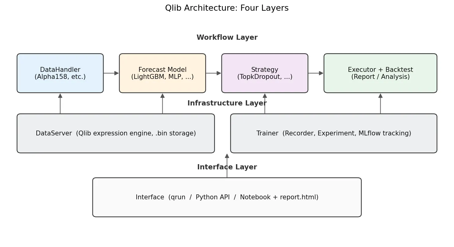
- DataServer is the bottom layer. It reads raw OHLCV from
.bincolumns and runs an expression engine. A string likeMean($close, 5)gets parsed into a 5-day rolling mean over close. - DataHandler turns raw data into
(features, labels)ready for ML training. Alpha158 is a built-in DataHandler with 158 expressions hardcoded. - Model is pure ML. Built-ins include LightGBM, XGBoost, MLP, LSTM, GRU, Transformer, Localformer, TCN, TabNet, ADD, ADARNN, HIST, all behind a uniform
fit(dataset)/predict(dataset)interface. - Strategy + Executor turns prediction scores into positions and orders, then replays them against historical prices. The most common one is
TopkDropoutStrategy, covered below. - Recorder/Analyser handles MLflow-style experiment tracking. Every
qrunsaves predictions, positions, and an HTML report.
The DataHandler internals are worth a closer look:
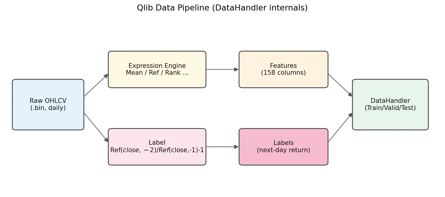
Raw .bin data flows in, the expression engine computes 158 feature columns, the label expression computes labels, then everything splits into train/valid/test for the model.
The default label is Ref($close, -2)/Ref($close, -1) - 1. Negative offsets mean future in Qlib: Ref($close,-1) is T+1 close and Ref($close,-2) is T+2 close, so this label is the T+1-close to T+2-close return. With TopkDropoutStrategy and deal_price=close, the workflow is: decide on day T using features that include T close, place orders for T+1 close fill. The earliest you can trade is T+1 close, never intra-day T. Any implementation that uses day-T features for a day-T fill leaks future information.
Inside the Alpha158 Factor Set
Alpha158 is the default factor set, defined in qlib/contrib/data/handler.py and qlib/contrib/data/loader.py. The 158 factors break down by construction type:
| Family | Example expression | Meaning |
|---|---|---|
| KBAR (candlestick, 9) | ($close-$open)/$open | Daily return, body/shadow ratios |
| ROC / MA (momentum, MA deviation) | Mean($close,5)/$close, Ref($close,5)/$close | 5/10/20/30/60-day windows |
| STD / BETA / RSQR / RESI (volatility, regression residuals) | Std($close/Ref($close,1)-1, 20) | Return vol, residual vs market |
| MAX / MIN / QTLU / QTLD (extrema and quantiles) | Max($high, 20)/$close | Distance to N-day high/low, quantile position |
| RANK / RSV (time-series rank, position-in-range) | Rank($close, 5) | Where today’s close sits in the last N days |
| IMAX / IMIN / IMXD (timing of extrema) | IdxMax($high, 20)/20 | How many days since the high |
| CORR / CORD (price-volume correlation) | Corr($close, Log($volume+1), 5) | Price vs log-volume correlation |
| CNTP / CNTN / CNTD / SUMP / SUMN / SUMD (up/down counting, signed sums) | Mean($close>Ref($close,1), 20) | Fraction of up days in last 20 |
| Volume family (VMA, VSTD, WVMA, VSUMP, …) | Std($volume, 20)/$volume | Volume volatility, weighted MAs |
Naming convention is <operator><window>: MA5 is the 5-day MA ratio, STD20 the 20-day volatility ratio, ROC10 the 10-day rate of change. To list all of them:
from qlib.contrib.data.loader import Alpha158DL
fields, names = Alpha158DL.get_feature_config()
for f, n in zip(fields, names):
    print(f"{n:12s} = {f}")
Faster than reading the docs.
After a few real runs the truth becomes clear: contributions across the 158 factors are wildly uneven. In my own CSI300 experiments the momentum family (ROC and MA-deviation factors) carries more than half of the total IC, the 9 KBAR candlestick factors trend toward zero IC, and the volume-price correlation block (CORR, CORD) is mostly noise on its own. LightGBM feature importance ranks line up with this. Treat Alpha158 as a baseline, but do not assume all 158 factors are pulling weight; in practice your model is leaning on maybe 30-50 of them.
Note also that everything in Alpha158 is derived from OHLCV. No fundamentals, no sentiment, no macro. For fundamentals you write your own DataHandler.
Running the Standard Workflow with qrun and YAML
Scripts are good for exploration, but YAML config plus qrun is better for paper reproduction and batch experiments. The Qlib repo ships examples/benchmarks/LightGBM/workflow_config_lightgbm_Alpha158.yaml as a complete template:
qlib_init:
    provider_uri: "~/.qlib/qlib_data/cn_data"
    region: cn

market: &market csi300
benchmark: &benchmark SH000300

data_handler_config: &data_handler_config
    start_time: 2008-01-01
    end_time: 2020-08-01
    fit_start_time: 2008-01-01
    fit_end_time: 2014-12-31
    instruments: *market

task:
    model:
        class: LGBModel
        module_path: qlib.contrib.model.gbdt
        kwargs:
            loss: mse
            colsample_bytree: 0.8879
            learning_rate: 0.0421
            subsample: 0.8789
            lambda_l1: 205.6999
            lambda_l2: 580.9768
            max_depth: 8
            num_leaves: 210
            num_threads: 20

    dataset:
        class: DatasetH
        module_path: qlib.data.dataset
        kwargs:
            handler:
                class: Alpha158
                module_path: qlib.contrib.data.handler
                kwargs: *data_handler_config
            segments:
                train: [2008-01-01, 2014-12-31]
                valid: [2015-01-01, 2016-12-31]
                test:  [2017-01-01, 2020-08-01]

    record:
        - class: SignalRecord
          module_path: qlib.workflow.record_temp
        - class: SigAnaRecord
          module_path: qlib.workflow.record_temp
        - class: PortAnaRecord
          module_path: qlib.workflow.record_temp
          kwargs:
              config:
                  strategy:
                      class: TopkDropoutStrategy
                      module_path: qlib.contrib.strategy
                      kwargs:
                          topk: 50
                          n_drop: 5
                  backtest:
                      start_time: 2017-01-01
                      end_time: 2020-08-01
                      account: 100000000
                      benchmark: *benchmark
                      exchange_kwargs:
                          freq: day
                          limit_threshold: 0.095
                          deal_price: close
                          open_cost: 0.0005
                          close_cost: 0.0015
                          min_cost: 5
Run it:
qrun workflow_config_lightgbm_Alpha158.yaml
You get a fresh experiment under mlruns/ with pred.pkl (predictions), port_analysis_1day.pkl (portfolio metrics), and a report.html with plotly charts: net value curve, excess return, rolling Sharpe, max drawdown. Open it in any browser.
The YAML anchor trick (&market / *market) is a Qlib config idiom worth noting. It avoids restating the universe and date ranges in three places (train, test, backtest); change once, and everything stays consistent.
Writing Your Own Alpha Expressions
The expression language is the heart of Qlib. Any OHLCV field gets a $ prefix ($close, $volume, $high), and operators follow a talib-like naming (Mean, Std, Ref, Rank, Corr, Cov, Sum, Min, Max, Abs, Log, Sign, Greater, Less, If).
A few examples:
| Expression | Meaning |
|---|---|
Mean($close, 5) | 5-day MA of close |
Ref($close, 1) | Yesterday’s close (lag 1) |
($close - Ref($close, 5)) / Ref($close, 5) | 5-day return |
Std($close/Ref($close,1)-1, 20) | 20-day return volatility |
Rank(Mean($volume, 5)/Mean($volume, 60)) | Cross-sectional rank of short/long volume ratio |
Corr($close, $volume, 10) | 10-day price-volume correlation |
Note Rank is cross-sectional (ranks across all instruments on a given day); the others are time-series rolling by default. This is the biggest difference from the WorldQuant Alpha syntax (see WorldQuant Alpha 101 Explained).
The simplest way to define a custom factor set is to subclass DataHandlerLP:
from qlib.data.dataset.handler import DataHandlerLP
from qlib.data.dataset.loader import QlibDataLoader

class MyHandler(DataHandlerLP):
    def __init__(self, instruments="csi300",
                 start_time=None, end_time=None,
                 fit_start_time=None, fit_end_time=None, **kwargs):
        feature_fields = [
            "Mean($close, 5)/$close - 1",
            "Mean($close, 20)/$close - 1",
            "Std($close/Ref($close,1)-1, 20)",
            "Corr($close, Log($volume+1), 10)",
        ]
        feature_names = ["ma5_dev", "ma20_dev", "vol20", "pv_corr10"]
        label_fields = ["Ref($close, -2)/Ref($close, -1) - 1"]
        label_names = ["LABEL0"]

        data_loader = {
            "class": "QlibDataLoader",
            "kwargs": {
                "config": {
                    "feature": (feature_fields, feature_names),
                    "label":   (label_fields, label_names),
                },
            },
        }
        super().__init__(
            instruments=instruments,
            start_time=start_time, end_time=end_time,
            data_loader=data_loader,
            fit_start_time=fit_start_time, fit_end_time=fit_end_time,
            **kwargs,
        )
Four factors is enough to validate an idea quickly.
Backtesting and Reading Performance: TopkDropout, IC, and ICIR
Qlib’s default TopkDropoutStrategy is simple but effective. The logic: each day, rank instruments by predicted score, hold the top K, and on the next day drop N names that fall out of the top region, replacing them with new entrants from the top.
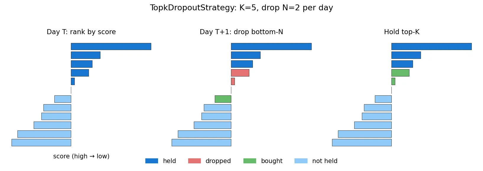
Why not full rotation every day? Turnover would eat all the alpha through transaction costs. n_drop controls turnover. K=50, n_drop=5 corresponds to roughly 10% daily turnover, a typical institutional setting.
Key metrics in the backtest output:
| Metric | Meaning | Reasonable range |
|---|---|---|
| IC | Pearson correlation between predicted and realised return | 0.02-0.08 normal for daily A-share |
| Rank IC | Spearman rank correlation, more robust | Usually slightly higher than IC |
| ICIR | Mean(IC) / Std(IC), stability measure | > 0.3 is good |
| Annualised return | Total annualised | 10%-25% is common |
| Excess annualised | Minus benchmark (CSI300) | Has to be positive to matter |
| Max drawdown | Worst cumulative loss | -20% to -40% is normal for A-share |
| Sharpe | Return / volatility | > 1 is workable, > 2 is rare |
A trap newcomers fall into: seeing IC 0.05, annual return 30%, Sharpe 2.5 and getting excited. Check a few things first. Is the test segment actually outside the training range (lookahead bias)? Alpha158’s label is Ref($close,-2)/Ref($close,-1)-1, the T+1-close-to-T+2-close return; the decision point is end-of-day T, earliest fill is T+1 close. If your custom strategy somehow lets a T-day decision execute intra-day T, you have leaked future information (more on this in Common Backtesting Pitfalls). Qlib’s defaults are clean, but when you write custom labels, count the Ref offsets carefully.
Common Errors and Pitfalls
By frequency from real-world use, these are the things any honest Qlib tutorial should warn you about:
1. FileNotFoundError: ... cn_data/calendars/day.txt not found
Wrong provider_uri in qlib.init, or ~ not expanding in your shell. Use an absolute path. Windows shells are particularly inconsistent about ~.
2. ValueError: instruments csi300 not found
Incomplete data download, or a region mismatch with provider_uri. Check ~/.qlib/qlib_data/cn_data/instruments/ for csi300.txt; if missing, re-run get_data.
3. Cannot allocate memory during LightGBM training
Alpha158 on the full CSI300 produces a roughly (1.5M, 158) feature matrix, peaking at 6-8 GB RAM. Fine on a desktop, tight on small cloud instances. Bump RAM, or shrink instruments to csi100, or push start_time forward.
4. MLP/GRU loss not decreasing
Qlib’s built-in neural networks (e.g. qlib.contrib.model.pytorch_general_nn.GeneralPTNN) do not normalise Alpha158 features by default, but the 158 factors span several orders of magnitude. Add processors like RobustZScoreNorm or CSZScoreNorm to the DataHandler. LightGBM does not need this, which is why most tutorials start with LightGBM.
5. Updating data to today
The official get_data archive lags by months. To catch up to yesterday:
# pull A-share delta to CSV via akshare collector
python scripts/data_collector/akshare/collector.py download_data \
    --source_dir ~/qlib_raw/cn --region cn --delay 1

# convert to .bin columnar format
python scripts/dump_bin.py dump_all \
    --csv_path ~/qlib_raw/cn \
    --qlib_dir ~/.qlib/qlib_data/cn_data \
    --include_fields open,close,high,low,volume,factor
--factor is the adjustment factor column. Skip it and your predictions get polluted by dividends and splits. First full run takes 1-2 hours; subsequent deltas finish in minutes.
6. qrun says mlflow.exceptions.MlflowException: Run ... not found
The mlruns/ directory was deleted manually or has permission issues. Wipe mlruns/0/ leftovers and rerun.
7. Non-ASCII paths on Windows
Put your data at D:/qlib_data/, not D:/我的数据/. Some C extensions in Qlib have bugs with non-ASCII paths.
Where to Go Next: RL, Rolling Training, RD-Agent
Once the entry-level path is comfortable, several directions are worth digging into:
Rolling training: in production, models cannot be trained once and used for three years. Market regimes drift. Qlib’s qlib.workflow.task.collect and RollingGen provide month-by-month or quarter-by-quarter retraining utilities.
RL for order execution: the qlib.rl module supports child-order RL strategies, with PPO and OPDS implementations. Reproduction code is in examples/rl_order_execution/.
RD-Agent: Microsoft’s July 2024 release at github.com/microsoft/RD-Agent, an LLM-driven automated factor mining system that uses Qlib as its execution environment. The LLM proposes new factors, runs experiments, reads results, and iterates. This is the most active direction in the Qlib ecosystem right now; related paper notes are at AlphaAgent paper review and AlphaGPT paper review.
Point-in-Time data: fundamental data has an announcement lag. Qlib’s PIT database supports point-in-time queries by announcement timestamp, which prevents the standard look-ahead bias in fundamental backtests.
That covers the entry path. If you followed it end-to-end, you have already done more than 90% of the “qlib tutorial” content out there. The two things that actually open up serious work from here: writing your first batch of custom factors on a universe you care about and running rolling retraining to test stability across regimes, and plugging RD-Agent in to let an LLM brute-force the factor combinatorics for you. I will cover both in follow-ups: rolling training plus akshare incremental updates, and an RD-Agent + Qlib factor-mining walkthrough. Subscribe via RSS or check back for the next post.