The core logic of pairs trading is straightforward: find two stocks whose prices “should move together,” and when they diverge from their historical relationship, bet on convergence. Go long the relatively cheap one, short the relatively expensive one, close when the spread reverts. You are not betting on market direction. You are betting on the relative pricing between two assets returning to normal.
Why Cointegration, Not Correlation
The most common beginner mistake in pairs trading: using correlation to find pairs. Two stocks with a 0.95 correlation over the past year look like a perfect pair. The problem is that high correlation does not mean the spread will revert.
Consider two stocks in the same sector, both up 40% over the past year, correlation 0.95. But stock A outpaces stock B by 0.5% every month. By year-end, A has cumulatively outperformed B by 6%. The correlation remains high (they move up and down together), but the spread is persistently widening. A pairs trader waiting for convergence will wait forever.
Correlation measures “do two series move in the same direction.” Cointegration measures “is a linear combination of two series stationary.” Stationary means mean-reverting: when the spread deviates, it gets pulled back.
The classic analogy: a drunk and his dog. Each wanders randomly on their own (non-stationary), but the leash keeps them bound together. The distance between them (the spread) is stationary and cannot grow without limit. Pairs trading bets that the “leash” exists.
Mathematically: two I(1) series \(X_t\) and \(Y_t\) are cointegrated if there exists a constant \(\beta\) such that \(Y_t - \beta X_t\) is I(0) (stationary).
Cointegration Testing: Engle-Granger Two-Step Method
The most common cointegration test is the Engle-Granger two-step method:
Step 1: Run OLS regression of \(Y\) on \(X\), obtaining the hedge ratio \(\hat{\beta}\) and residual series \(e_t = Y_t - \hat{\beta} X_t\).
Step 2: Run an ADF (Augmented Dickey-Fuller) test on the residuals \(e_t\). If the ADF p-value is below the threshold (typically 0.05), reject the null hypothesis of a unit root in the residuals, concluding that the residuals are stationary and the two series are cointegrated.
Using yfinance for data, here is the complete implementation:
import numpy as np
import yfinance as yf
from statsmodels.tsa.stattools import adfuller
from sklearn.linear_model import LinearRegression

# Download data
tickers = ["KO", "PEP"]  # Coca-Cola vs PepsiCo
data = yf.download(tickers, start="2023-01-01", end="2024-12-31")["Close"]
data = data.dropna()

X = data["KO"].values.reshape(-1, 1)
Y = data["PEP"].values

# Step 1: OLS regression
reg = LinearRegression().fit(X, Y)
beta = reg.coef_[0]
intercept = reg.intercept_
spread = Y - beta * X.flatten() - intercept

print(f"Hedge ratio beta = {beta:.4f}")
print(f"Intercept = {intercept:.4f}")

# Step 2: ADF test
adf_result = adfuller(spread, autolag="AIC")
print(f"ADF statistic: {adf_result[0]:.4f}")
print(f"p-value: {adf_result[1]:.4f}")
print(f"Conclusion: {'Cointegrated' if adf_result[1] < 0.05 else 'Not cointegrated'}")
Using KO/PEP as an example, typical output looks like:
Hedge ratio beta = 2.9477
Intercept = -3.8326
ADF statistic: -3.9587
p-value: 0.0016
Conclusion: Cointegrated
The ADF p-value is well below 0.05, confirming that the KO/PEP spread is stationary. The hedge ratio β ≈ 2.95 means for every 1 share of PEP long, you need to short approximately 2.95 shares of KO to hedge.
A few practical notes:
Sample selection: 2-3 years of daily data is standard. Too short (6 months) gives insufficient sample size and low ADF test power. Too long (10 years) may span regime changes where the cointegration relationship held early but has since broken down.
Pair candidates: Do not blindly search all stock combinations. Pre-filter candidates using sector logic (same industry, same supply chain, similar ETFs), then validate with cointegration tests. Searching all pairs among 5,000 stocks (12.5 million combinations) will produce numerous spurious cointegration results (multiple testing problem).
Johansen test: If you want to test cointegration among three or more stocks simultaneously, Engle-Granger is insufficient. The Johansen test can identify multiple cointegrating vectors, making it suitable for basket trading.
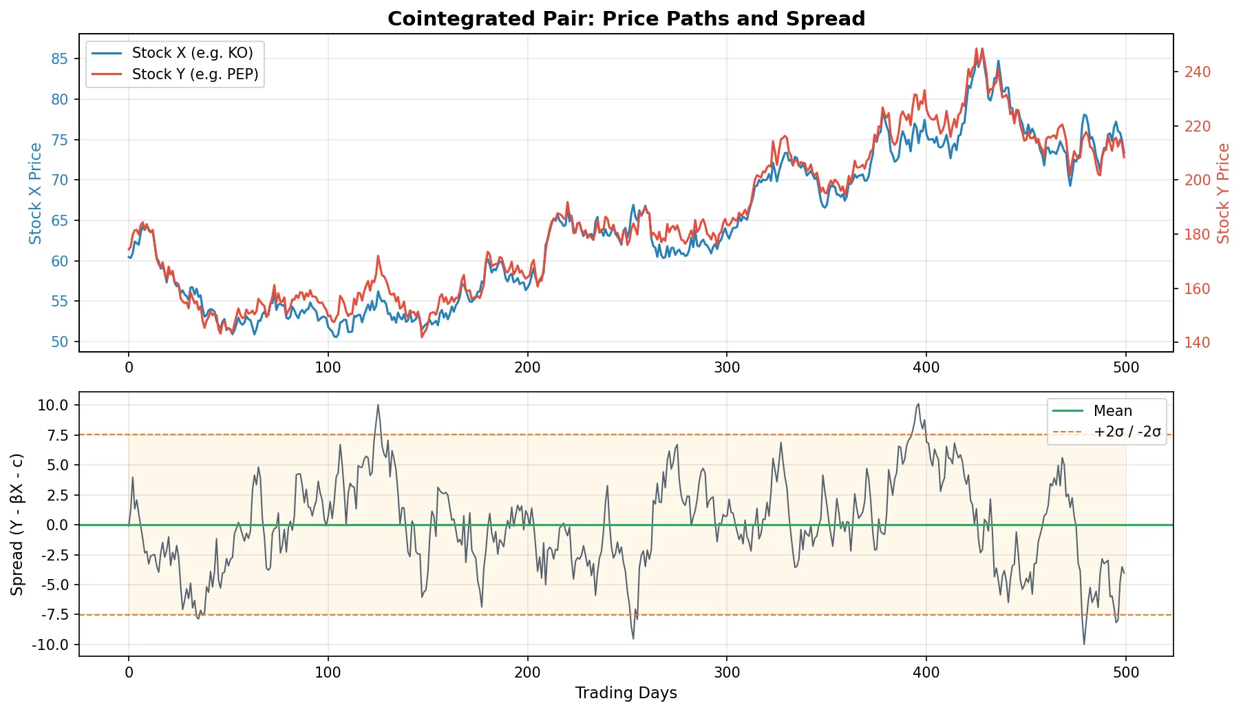
Spread Construction
After cointegration is confirmed, the next step is constructing a tradeable spread.
$$\text{spread}_t = Y_t - \beta X_t - c$$where \(\beta\) is the hedge ratio (OLS slope) and \(c\) is the intercept. This spread should be stationary and mean-reverting.
Rolling window vs. full sample: The \(\beta\) above uses the full-sample regression, but cointegration relationships are not static. The hedge ratio drifts slowly over time. In practice, use a rolling window (e.g., 60 trading days) to dynamically update \(\beta\):
def rolling_hedge_ratio(Y, X, window=60):
    """Compute hedge ratio using a rolling window"""
    betas = np.full(len(Y), np.nan)
    for i in range(window, len(Y)):
        reg = LinearRegression().fit(X[i-window:i].reshape(-1, 1), Y[i-window:i])
        betas[i] = reg.coef_[0]
    return betas
Z-score normalization: Convert the spread to a standardized score for threshold-based trading.
$$Z_t = \frac{\text{spread}_t - \overline{\text{spread}}}{\text{std}(\text{spread})}$$The mean and standard deviation are also computed on a rolling basis. A Z-score above 2 indicates the spread has deviated by 2 standard deviations, a potential entry signal.
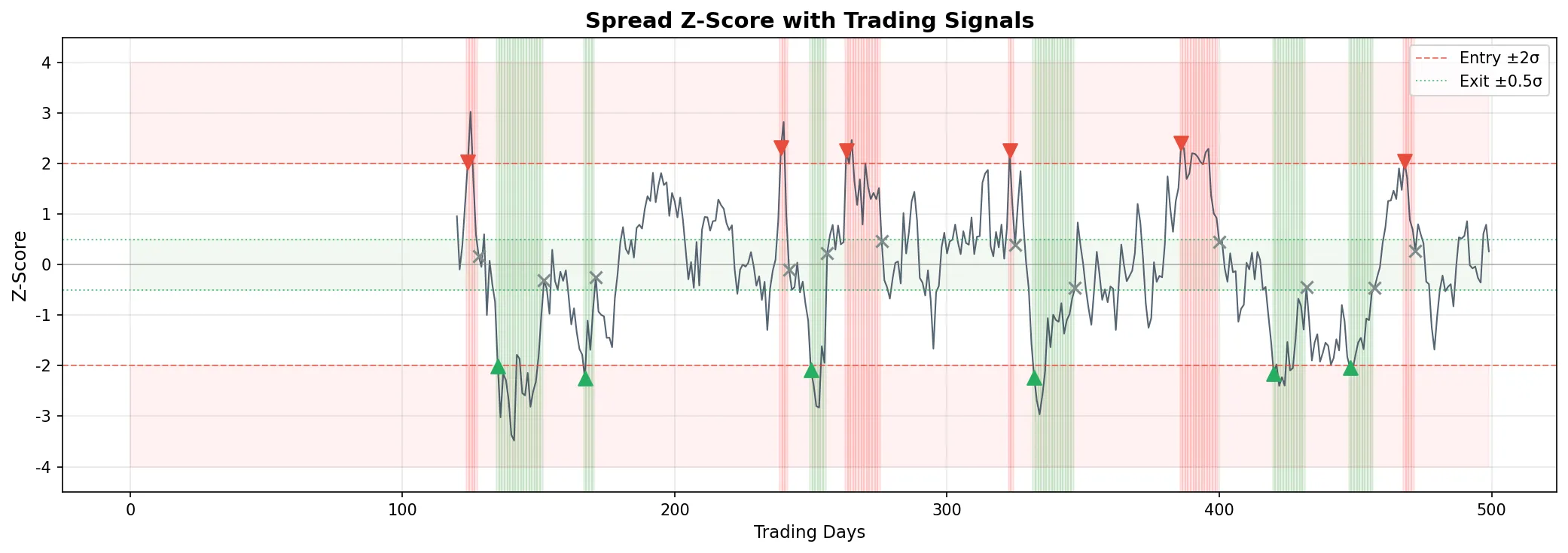
Trading Signals and Backtesting
Classic mean-reversion signals:
| Z-score Condition | Action |
|---|---|
| Z > +2 | Short the spread (short Y, long \(\beta\) units of X) |
| Z < -2 | Long the spread (long Y, short \(\beta\) units of X) |
| |Z| < 0.5 | Close position (spread has reverted) |
| |Z| > 4 | Stop loss (spread still diverging, cointegration may be broken) |
Complete signal generation and simplified backtest:
import numpy as np
import yfinance as yf
from sklearn.linear_model import LinearRegression

# Data preparation
data = yf.download(["KO", "PEP"], start="2023-01-01", end="2024-12-31")["Close"].dropna()
Y = data["PEP"].values
X = data["KO"].values

# Rolling parameters
lookback = 60
start = 2 * lookback  # first 2*lookback days used for warm-up

# Compute rolling spread and Z-score
spread = np.full(len(Y), np.nan)
z_score = np.full(len(Y), np.nan)

for i in range(lookback, len(Y)):
    reg = LinearRegression().fit(X[i-lookback:i].reshape(-1, 1), Y[i-lookback:i])
    beta = reg.coef_[0]
    spread[i] = Y[i] - beta * X[i] - reg.intercept_

# Z-score from rolling mean and std of the spread itself
for i in range(start, len(Y)):
    window = spread[i-lookback:i]
    valid = window[~np.isnan(window)]
    if len(valid) >= 20 and np.std(valid) > 0:
        z_score[i] = (spread[i] - np.mean(valid)) / np.std(valid)

# Generate signals
position = np.zeros(len(Y))  # +1 = long spread, -1 = short spread
for i in range(start + 1, len(Y)):
    if np.isnan(z_score[i]):
        position[i] = position[i-1]
        continue
    if position[i-1] == 0:
        if z_score[i] > 2:
            position[i] = -1       # short spread
        elif z_score[i] < -2:
            position[i] = +1       # long spread
    elif position[i-1] == 1:       # currently long spread (entered at Z<-2)
        if abs(z_score[i]) < 0.5:  # spread reverted, close
            position[i] = 0
        elif z_score[i] < -4:      # spread diverging further, stop loss
            position[i] = 0
        else:
            position[i] = 1
    elif position[i-1] == -1:      # currently short spread (entered at Z>+2)
        if abs(z_score[i]) < 0.5:  # spread reverted, close
            position[i] = 0
        elif z_score[i] > 4:       # spread diverging further, stop loss
            position[i] = 0
        else:
            position[i] = -1

# Simplified P&L (daily spread change x position)
spread_ret = np.diff(spread)
daily_pnl = position[start:-1] * spread_ret[start-1:]
daily_pnl = daily_pnl[~np.isnan(daily_pnl)]
cumulative_pnl = np.cumsum(daily_pnl)

n_trades = int(np.sum(np.abs(np.diff(position[start:])) > 0))
print(f"Total P&L: {cumulative_pnl[-1]:.2f}")
print(f"Number of trades: {n_trades}")
print(f"Daily mean P&L: {np.mean(daily_pnl):.4f}")
print(f"Annualized Sharpe: {np.mean(daily_pnl) / np.std(daily_pnl) * np.sqrt(252):.2f}")
Running this on KO/PEP 2023-2024 data, typical results:
Total P&L: 46.07
Number of trades: 24 (12 round trips)
Daily mean P&L: 0.1215
Annualized Sharpe: 2.19
12 round-trip trades, annualized Sharpe of 2.19. Looks good, but note: the strategy is only in a position 27% of the time (the spread stays within ±2σ most of the time), no transaction costs are deducted, and margin requirements for both legs are ignored. The real Sharpe would be meaningfully lower.
This backtest is heavily simplified: no transaction costs, no slippage, no capital allocation modeling. Real performance will be worse.
Risks and Limitations
Cointegration relationships break. This is the biggest risk in pairs trading. Two stocks cointegrated over the past 3 years does not guarantee future cointegration. Changes in company fundamentals (mergers, business pivots, regulatory shifts) can permanently break the relationship. In practice, monitor continuously: re-run the ADF test periodically (e.g., monthly), and if the p-value rises above 0.10, consider closing the pair.
Execution risk. Pairs trading requires simultaneously buying one stock and selling another. If both legs cannot be filled simultaneously, the delay creates directional exposure. Illiquid stocks are especially dangerous: you may fill one leg only to find the other leg’s price has already moved.
Capital efficiency. Going long one stock and short another ties up margin or capital on both legs. Compared to single-leg strategies, pairs trading has lower capital utilization. Using the Kelly Criterion to size each pair optimally can help allocate capital across multiple pairs.
Uncertain convergence timing. A spread 2 standard deviations from the mean might revert tomorrow or two months from now. During the holding period, capital is locked up, and the opportunity cost is a hidden drag on returns.
Overfitting risk in backtesting. Pairs trading backtests are especially prone to overfitting. Screening 5,000 stocks to find pairs that pass the cointegration test is a form of data mining. The solution is strict out-of-sample validation: use the first 2 years to identify pairs, the third year to validate, and only trade pairs that also pass cointegration out-of-sample.
Pairs trading strategies typically produce Sharpe ratios between 1.0 and 2.0. Not exceptional, but the appeal lies in stability and market neutrality.