The first two articles covered first-order Greeks and second-order Greeks, building up the math, the intuition, and the code. This article does one thing: use those numbers to make trading decisions. What Greeks profile does each strategy carry? How does Delta hedging actually work in discrete time? When does Gamma Scalping have positive expected value? How do market makers use Greeks for risk management? Numbers and code throughout.
This is the final article in the Option Greeks series.
Decomposing Strategies with Greeks
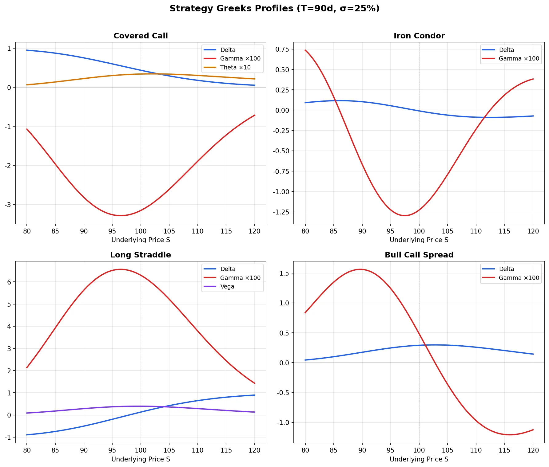
Options strategies come in hundreds of varieties, but Greeks reduce them to four or five risk types. The analysis below uses standard parameters: S=100, K=100, T=0.25, σ=25%, r=5%.
Covered Call: Selling Upside for Theta
Hold 100 shares + sell 1 ATM call contract.
| Greek | Stock | Short Call | Net Position |
|---|---|---|---|
| Delta | +1.00 | -0.56 | +0.44 |
| Gamma | 0 | -0.031 | -0.031 |
| Theta | 0 | +0.034 | +0.034 |
| Vega | 0 | -0.197 | -0.197 |
The trade: you collect $0.034/day in Theta income. You pay for it by capping upside above the strike, taking on negative Vega (IV rise hurts), and negative Gamma (large moves hurt). This fits a view that the underlying will trade sideways to slightly higher.
Iron Condor: Range-Bound Theta Harvesting
Sell K=95 put + buy K=90 put + sell K=105 call + buy K=110 call.
The Greeks profile is distinctive:
- Delta ≈ 0: Symmetric on both sides, directionally neutral
- Gamma < 0: Large moves in either direction are the enemy
- Theta > 0: Daily Theta collection is the income source
- Vega < 0: IV decline helps, IV rise hurts
Iron Condor traders often say “as long as the stock stays in the range, we make money.” This is only half right. Even if the stock stays in range, a 10-point IV spike causes meaningful mark-to-market losses through negative Vega before the options expire. Greeks let you quantify “how much do I lose if IV spikes 10 points” rather than discovering it after the fact.
Long Straddle: Buying Volatility
Buy ATM call + buy ATM put (same strike, same expiry).
| Greek | Long Call | Long Put | Net Position |
|---|---|---|---|
| Delta | +0.56 | -0.44 | +0.12 |
| Gamma | +0.031 | +0.031 | +0.063 |
| Theta | -0.034 | -0.020 | -0.054 |
| Vega | +0.197 | +0.197 | +0.394 |
A straddle is long two things: realized volatility (via positive Gamma) and implied volatility (via positive Vega). You pay $0.054/day in Theta, betting on either a large underlying move or an IV increase.
Net Delta is not zero (+0.12) due to the interest rate effect. In practice, many traders adjust the ratio slightly or add a small stock position to achieve approximate Delta neutrality.
Bull Call Spread: Bounded Directional Bet
Buy K=100 call + sell K=110 call.
- Delta +0.30: Bullish, but less aggressive than a naked call
- Gamma ≈ 0: The long and short call Gammas largely offset
- Theta ≈ 0: Long and short Theta also offset
- Vega ≈ 0: Same logic
Spreads use the sold leg to “subsidize” the bought leg, at the cost of capping profit potential. For spreads with highly asymmetric Greeks (like a calendar spread, selling near-month and buying far-month), the Greek interactions become much more complex.
Dynamic Delta Hedging: Theory Meets Reality
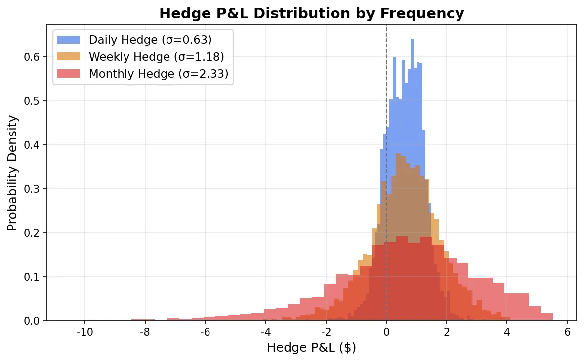
BSM assumes continuous rehedging: infinite frequency, zero transaction costs. Every real hedge trade incurs costs: commissions, bid-ask spread, market impact. This creates a core trade-off: higher hedge frequency reduces Gamma exposure but increases transaction costs.
The Python simulation below makes this trade-off visible. We generate underlying price paths using geometric Brownian motion (GBM) and compare the hedging P&L distribution across different rebalancing frequencies.
import numpy as np
from scipy.stats import norm

def simulate_delta_hedge(S0, K, T, r, sigma, n_steps, n_paths=5000, cost_per_trade=0.01):
    """
    Simulate Delta hedging P&L distribution
    S0: initial underlying price
    n_steps: number of hedge rebalances (more = higher frequency)
    cost_per_trade: transaction cost per share per rebalance
    """
    dt = T / n_steps
    np.random.seed(42)

    Z = np.random.randn(n_paths, n_steps)
    S = np.zeros((n_paths, n_steps + 1))
    S[:, 0] = S0
    for i in range(n_steps):
        S[:, i+1] = S[:, i] * np.exp((r - 0.5*sigma**2)*dt + sigma*np.sqrt(dt)*Z[:, i])

    d1_0 = (np.log(S0/K) + (r + 0.5*sigma**2)*T) / (sigma*np.sqrt(T))
    d2_0 = d1_0 - sigma*np.sqrt(T)
    option_premium = S0 * norm.cdf(d1_0) - K * np.exp(-r*T) * norm.cdf(d2_0)

    cash = option_premium * np.ones(n_paths)
    shares = np.zeros(n_paths)
    total_cost = np.zeros(n_paths)

    for i in range(n_steps):
        t_remaining = T - i * dt
        if t_remaining <= 0:
            break
        d1 = (np.log(S[:, i]/K) + (r + 0.5*sigma**2)*t_remaining) / (sigma*np.sqrt(t_remaining))
        delta = norm.cdf(d1)
        trade = delta - shares
        cash -= trade * S[:, i]
        total_cost += np.abs(trade) * cost_per_trade
        shares = delta

    payoff = np.maximum(S[:, -1] - K, 0)
    final_pnl = cash + shares * S[:, -1] - payoff - total_cost
    final_pnl *= np.exp(-r * T)
    return final_pnl

pnl_daily = simulate_delta_hedge(100, 100, 0.25, 0.05, 0.25, n_steps=63)
pnl_weekly = simulate_delta_hedge(100, 100, 0.25, 0.05, 0.25, n_steps=13)
pnl_monthly = simulate_delta_hedge(100, 100, 0.25, 0.05, 0.25, n_steps=3)

print(f"Daily hedge:   mean={pnl_daily.mean():.3f}, std={pnl_daily.std():.3f}")
print(f"Weekly hedge:  mean={pnl_weekly.mean():.3f}, std={pnl_weekly.std():.3f}")
print(f"Monthly hedge: mean={pnl_monthly.mean():.3f}, std={pnl_monthly.std():.3f}")
Key takeaways:
- Daily hedging has the tightest P&L distribution (smallest standard deviation) but slightly lower mean due to transaction costs
- Monthly hedging saves on costs but dramatically increases P&L variance; you bear much more Gamma risk
- The optimal frequency depends on Gamma magnitude, transaction costs, and your tolerance for P&L volatility
In practice, market makers typically do not hedge on a fixed schedule. They use a Delta bandwidth: rehedge only when net Delta exceeds a threshold. How to set the threshold? A rough guide is the Whalley-Wilmott bandwidth:
$$\Delta_{band} \approx \left(\frac{3}{2} \cdot \frac{\text{transaction cost} \cdot \Gamma}{\lambda}\right)^{1/3}$$where \(\lambda\) is a risk-aversion parameter. The intuition: higher Gamma (Delta changes fast) means a narrower bandwidth (hedge more often); higher transaction costs mean a wider bandwidth (trade less).
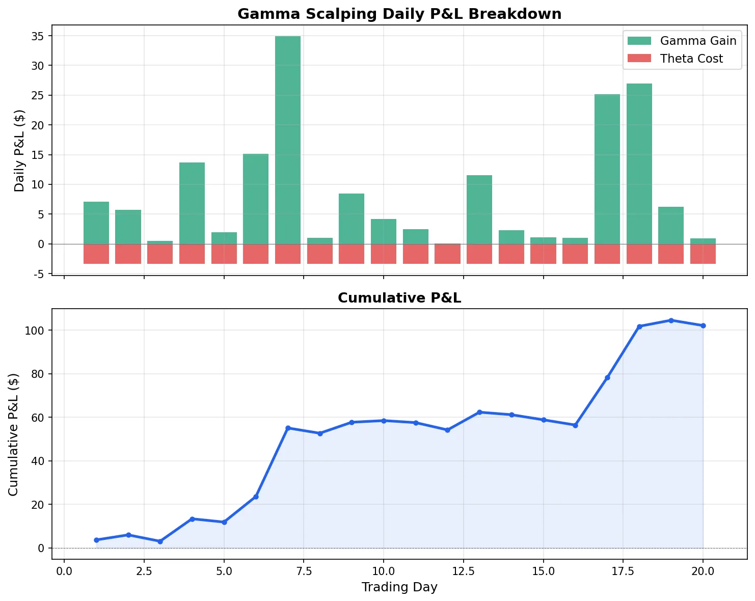
Gamma Scalping: Going Long Realized Volatility
Gamma Scalping is a core technique for market makers and volatility traders. The logic:
- Buy options (long Gamma, long Vega)
- Delta hedge to neutral
- After each significant underlying move, rehedge. Each rehedge “locks in” the Gamma convexity profit
- On quiet days, Theta erodes your account
P&L depends on one key comparison: realized volatility vs. implied volatility.
- Realized vol > implied vol → Gamma gains > Theta costs → profit
- Realized vol < implied vol → Gamma gains < Theta costs → loss
A simplified 5-day walkthrough (holding ATM call, Gamma=0.03, daily Theta=-$3.40 per contract):
| Day | Underlying | Move | Delta | Hedge Action | Gamma P&L | Theta Cost | Cumulative |
|---|---|---|---|---|---|---|---|
| 0 | 100.00 | — | 0.50 | Sell 50 shares | — | — | 0 |
| 1 | 102.50 | +2.50 | 0.575 | Sell 7.5 shares | +$9.38 | -$3.40 | +$5.97 |
| 2 | 99.00 | -3.50 | 0.47 | Buy 10.5 shares | +$18.38 | -$3.40 | +$20.95 |
| 3 | 99.50 | +0.50 | 0.485 | Sell 1.5 shares | +$0.38 | -$3.40 | +$17.93 |
| 4 | 103.00 | +3.50 | 0.59 | Sell 10.5 shares | +$18.38 | -$3.40 | +$32.90 |
| 5 | 100.50 | -2.50 | 0.51 | Buy 8 shares | +$9.38 | -$3.40 | +$38.88 |
In this example, the underlying moves 2-3% daily, so realized vol exceeds the 25% implied vol and Gamma gains cover Theta costs. If the underlying only moved 0.5% daily, Gamma gains would fall far short of Theta, and the strategy would bleed.
The Gamma P&L formula: \(\text{Gamma P\&L} \approx \frac{1}{2} \Gamma (\Delta S)^2\). Theta cost is fixed daily, but Gamma gains scale with \((\Delta S)^2\). This is why Gamma Scalping is “going long realized volatility.”
Practical details often overlooked:
Hedge timing: Theory says hedge after every move, but over-hedging gets eaten by transaction costs. Many Gamma Scalpers use fixed Delta thresholds or fixed time intervals (e.g., rehedge once at the close).
Gamma is not constant: After a large move, Gamma itself changes (this is Speed), making the next hedge quantity estimate inaccurate. This effect is especially pronounced near expiry.
Entry cost: You buy at implied vol and harvest realized vol. If IV collapses during your holding period (IV Crush), even if realized vol equals implied vol, you can lose money. Vega losses stack on top.
Vega Trading and IV Arbitrage
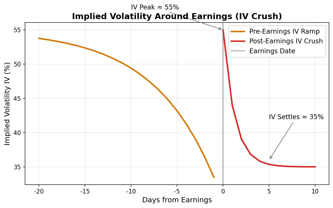
Earnings IV Crush Strategy
IV typically gets bid up before earnings. Suppose a stock’s normal IV is 30%, rising to 55% the week before earnings. After the report, IV collapses to 35%.
Short straddle for IV Crush: Sell ATM call + ATM put. Portfolio Vega = -0.40. IV drops from 55% to 35%, so Vega alone generates 0.40 × 20 = $8.00 profit. But the underlying also moves, and an 8% post-earnings gap can eat most of the Vega gains through Gamma losses.
So earnings trading is not as simple as “IV always drops, so sell straddles.” You need to compare: expected IV Crush magnitude × Vega, vs. expected underlying move magnitude × Gamma-driven losses. The market’s “Expected Move” is precisely the pricing of this balance point.
Calendar Spread: Playing Near-vs-Far Vega
Buy far-month call + sell near-month call (same strike). The near-month option has smaller Vega, the far-month has larger Vega, so net Vega is positive.
This strategy bets on IV term structure changes. If short-term IV drops (near-month Theta gain) while long-term IV stays flat or rises (far-month Vega gain), the calendar spread wins on both ends. The risk: if IV drops across the board, the far-month Vega loss exceeds the near-month Vega gain, because far-month Vega is larger.
Greeks Risk Management: The Market-Maker View
Market makers do not manage Greeks position by position. They aggregate the entire book’s Greeks and manage at the portfolio level.
Portfolio-Level Greeks Aggregation
With 200 positions across different strikes and expiries, each with its own Delta, Gamma, Theta, and Vega, portfolio-level Greeks are simple sums (Greeks are linear):
$$\Delta_{portfolio} = \sum_{i=1}^{n} w_i \cdot \Delta_i, \quad \Gamma_{portfolio} = \sum_{i=1}^{n} w_i \cdot \Gamma_i$$where \(w_i\) is the contract count for position \(i\) (positive = long, negative = short).
Greek Limits
Market makers set caps on each Greek:
| Greek | Typical Limit | Meaning |
|---|---|---|
| Net Delta | ±$500K share equivalents | Maximum directional exposure |
| Net Gamma | ±$50K per 1% move | Maximum P&L impact from large moves |
| Net Vega | ±$100K per 1 vol point | Maximum P&L impact from IV changes |
| Net Theta | Monitored, not hard-capped | Daily time decay income/cost |
When a limit is breached, the trader must reduce or hedge within a deadline. This is why market makers sometimes close positions at seemingly unfavorable prices: not because their view changed, but because a Greek limit was hit.
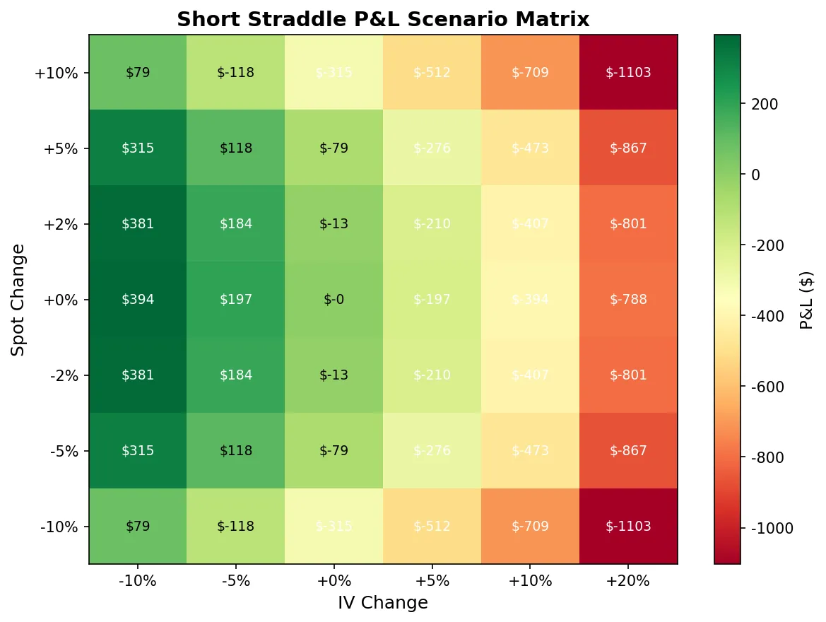
Scenario Analysis
Individual Greeks are insufficient. The real risk is multiple variables moving simultaneously. Market makers use a Scenario Matrix:
| Spot Δ \ IV Δ | IV -5% | IV flat | IV +5% | IV +10% | IV +20% |
|---|---|---|---|---|---|
| -10% | ? | ? | ? | ? | ? |
| -5% | ? | ? | ? | ? | ? |
| Flat | ? | ? | 0 | ? | ? |
| +5% | ? | ? | ? | ? | ? |
| +10% | ? | ? | ? | ? | ? |
Each cell: “if the underlying moves X% and IV moves Y points, what is portfolio P&L?” The matrix instantly reveals the most dangerous scenarios.
The February 2018 VIX spike is the definitive case study for scenario analysis failure. Many funds were short VIX futures and options (short Gamma + short Vega), collecting Theta daily. Their scenario matrices had a “VIX doubles in one day” cell showing catastrophic losses, but they judged this scenario “impossible.” On February 5th, VIX surged from 17 to 37 and XIV (inverse VIX ETN) went to zero overnight. A negative Gamma + negative Vega portfolio under a vol spike takes damage from two directions simultaneously: the underlying moves more (negative Gamma hurts), and vol rises (negative Vega hurts).
The lesson is direct: the corners of your scenario matrix that you label “impossible” are precisely the scenarios that define your risk. Market makers bound the P&L in those extreme cells to survivable levels, not because they expect those scenarios, but because survival is the prerequisite for everything else.
Series Summary
Three articles covering option Greeks from theory to practice:
- Part 1: First-order Greeks formulas, intuition, and code, answering “how much do I make if the stock moves $1?”
- Part 2: Second-order Greeks and the volatility surface, answering “why did my hedge drift overnight?”
- Part 3 (this article): Trading applications, answering “how do I use these numbers for trading and risk management?”
- Tool: Interactive Greeks calculator with real-time curve visualization
Greeks are not academic decoration. Market makers check Greeks before the open, monitor them in real-time during the session, and review them after the close. Trading options without watching Greeks is like driving without a dashboard.