The previous article covered the five first-order Greeks: Delta, Gamma, Theta, Vega, and Rho. They handle hedging and risk management well, with one assumption: the first-order Greeks themselves are stable. They are not. The underlying moves, and Delta changes (that is Gamma). Volatility shifts, and Delta changes again, but first-order Greeks have no name for this effect. Second-order Greeks fill that gap: they quantify the instability of first-order Greeks themselves.
This is part two of the Option Greeks series. It covers the three most important second-order Greeks (Vanna, Charm, Volga), plus their role in volatility surface modeling. Part three covers trading applications.
Why Second-Order Greeks Matter
First-order Greeks carry an implicit qualifier: “all else equal.” Delta tells you how much the option price moves for a $1 change in the underlying, but only if volatility, time, and rates stay fixed. In real trading, the underlying gaps 3%, IV spikes 5 points, and a day passes, all simultaneously. First-order approximations break down.
Second-order Greeks are derivatives of first-order Greeks. Mathematically, they are mixed or second partial derivatives of the option price. Under BSM, all of them have closed-form formulas, requiring no numerical differentiation.
| Second-Order Greek | Mathematical Definition | Intuitive Meaning |
|---|---|---|
| Vanna | \(\frac{\partial^2 V}{\partial S \partial \sigma}\) | When IV moves, how much does your Delta hedge shift? |
| Charm | \(\frac{\partial^2 V}{\partial S \partial T}\) | After one day passes, how much does your Delta drift? |
| Volga (Vomma) | \(\frac{\partial^2 V}{\partial \sigma^2}\) | Vega’s convexity: Vega is not constant under large vol moves |
| Speed | \(\frac{\partial^3 V}{\partial S^3}\) | Rate of change of Gamma; source of hedging error in large moves |
| Color | \(\frac{\partial^3 V}{\partial S^2 \partial T}\) | How Gamma decays over time |
| Ultima | \(\frac{\partial^3 V}{\partial \sigma^3}\) | Rate of change of Volga; only relevant in extreme vol environments |
Why do market makers care? A portfolio of thousands of options positions, hedged to Delta neutral each morning, will have its net Delta drift by afternoon. Charm and Vanna push it silently. A market maker who only tracks first-order Greeks will find their “Delta neutral” portfolio is actually running naked exposure.
The Python code below extends the BSMCalculator from Part 1 with the three core second-order Greeks:
import numpy as np
from scipy.stats import norm

class BSMSecondOrder:
    """BSM second-order Greeks (extending first-order)"""

    def __init__(self, S, K, T, r, sigma):
        self.S = S
        self.K = K
        self.T = T
        self.r = r
        self.sigma = sigma
        self.d1 = (np.log(S / K) + (r + 0.5 * sigma**2) * T) / (sigma * np.sqrt(T))
        self.d2 = self.d1 - sigma * np.sqrt(T)

    def vanna(self):
        """dDelta/dSigma = dVega/dS"""
        d1, d2 = self.d1, self.d2
        return -norm.pdf(d1) * d2 / self.sigma

    def charm(self, option_type='call'):
        """dDelta/dT (note: decreasing T = time passing)"""
        d1, d2 = self.d1, self.d2
        S, K, T, r, sigma = self.S, self.K, self.T, self.r, self.sigma
        common = -norm.pdf(d1) * (2 * r * T - d2 * sigma * np.sqrt(T)) / (2 * T * sigma * np.sqrt(T))
        if option_type == 'call':
            return common
        return common + r * np.exp(-r * T) * norm.cdf(-d2)

    def volga(self):
        """d²V/dSigma² = Vega's convexity"""
        d1, d2 = self.d1, self.d2
        S, T, sigma = self.S, self.T, self.sigma
        vega = S * norm.pdf(d1) * np.sqrt(T)
        return vega * d1 * d2 / sigma

# Example: same parameters S=100, K=100, T=0.25, r=5%, sigma=25%
bsm2 = BSMSecondOrder(S=100, K=100, T=0.25, r=0.05, sigma=0.25)
print(f"Vanna:  {bsm2.vanna():.6f}")    # -0.059056
print(f"Charm:  {bsm2.charm():.6f}")    # -0.127956
print(f"Volga:  {bsm2.volga():.6f}")    #  0.479834
One common source of confusion: Charm’s sign. Charm is defined as \(\frac{\partial \Delta}{\partial T}\), where \(T\) is time-to-expiry. \(T\) decreasing means time is passing. So positive Charm means Delta increases as \(T\) shrinks (as time passes). Some references define Charm with respect to calendar time \(t\) (opposite direction from \(T\)), flipping the sign. The code above uses the \(T\) convention, consistent with most textbooks.
Vanna: How Volatility Shifts Your Delta
Vanna has an elegant symmetry: it is simultaneously the derivative of Delta with respect to volatility, and the derivative of Vega with respect to the underlying price.
$$\text{Vanna} = \frac{\partial \Delta}{\partial \sigma} = \frac{\partial \mathcal{V}}{\partial S} = -\frac{N'(d_1) \cdot d_2}{\sigma}$$This symmetry is not coincidence. It follows from Schwarz’s theorem (equality of mixed partials). But it yields two distinct trading insights:
Through the Delta lens: When IV spikes, your Delta hedge needs adjusting. Suppose you hold an OTM call (Delta = 0.25) with positive Vanna. IV suddenly jumps 10 points, and your Delta is no longer 0.25 but something higher. You have more directional exposure to the upside than you intended. Market makers discover during IV storms that their “Delta neutral” portfolios are suddenly anything but neutral, and Vanna tells them by how much.
Through the Vega lens: When the underlying rallies, your Vega exposure changes. An OTM option has less Vega than an ATM option. As the underlying moves toward the strike, Vega increases, and that is Vanna at work.
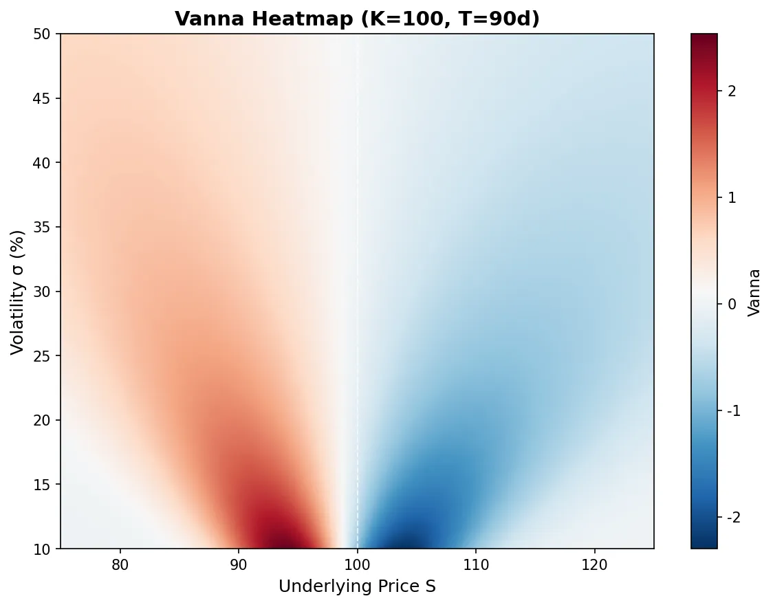
Vanna crosses zero near ATM, where ATM options’ Delta is relatively insensitive to volatility shifts (Vanna ≈ 0). Away from ATM, Vanna’s absolute value grows, and OTM/ITM options’ Delta becomes genuinely responsive to IV changes. This explains a real-world observation: an ATM straddle’s Delta stays relatively stable when IV moves, while OTM wings’ Deltas drift substantially.
Vanna in skew trading: When you trade a risk reversal (long OTM call + short OTM put), you are not just taking a directional view. If skew is steep (put IV far above call IV), the risk reversal carries significant Vanna exposure. A parallel IV shift moves the high-IV leg’s Delta more than the low-IV leg, and the portfolio’s net Delta drifts. Traders who ignore Vanna think they are running a pure directional trade; in reality, vol-of-vol risk has entered through the back door.
Charm: Overnight Delta Drift
$$\text{Charm} = \frac{\partial \Delta}{\partial T} = -N'(d_1) \cdot \frac{2rT - d_2 \sigma\sqrt{T}}{2T\sigma\sqrt{T}}$$Charm measures how much Delta changes purely from the passage of time; nothing else moves. You hedge to Delta neutral at the close. The underlying opens flat the next morning. Your net Delta has already shifted. By how much? Charm × 1 day.
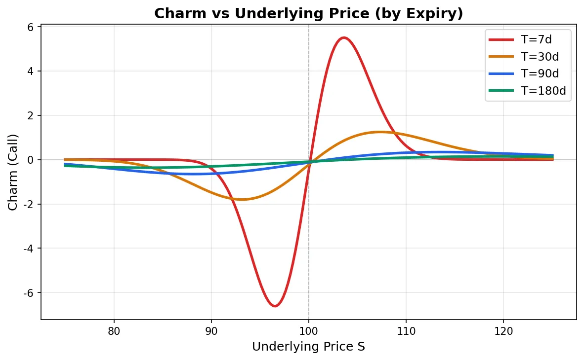
Charm’s profile relates to Gamma. ATM options tend to have large absolute Charm because ATM is where Delta changes fastest, so time’s push on Delta is strongest there. OTM call Charm is typically negative (Delta shrinks as time passes, since the option is increasingly likely to expire worthless). ITM call Charm is positive (Delta gravitates toward 1).
The Friday effect: From Friday’s close to Monday’s open spans the entire weekend. Market makers watch Charm closely on Friday afternoons because there is zero ability to rehedge over the weekend, yet Delta drifts silently for two days. A common scenario: you hold a large position in near-expiry OTM calls, Delta is manageable on Friday, and Monday morning Delta has dropped meaningfully because the options are closer to expiry, OTM probability increased. Without pre-adjusting for Charm before the weekend, you are gambling.
Charm becomes ferocious near expiry. Like Gamma, it diverges as \(T \to 0\). In the last day or two, ATM options’ Delta can visibly change every hour, not because the underlying is moving, but because time itself is pushing it.
Volga (Vomma): Vega’s Convexity
$$\text{Volga} = \frac{\partial^2 V}{\partial \sigma^2} = \mathcal{V} \cdot \frac{d_1 d_2}{\sigma}$$Volga measures how Vega itself responds to volatility changes. First-order analysis uses Vega to estimate “IV up 1 point, option price up X.” But what if IV moves 10 points? Is linear extrapolation reliable? Volga quantifies the deviation.
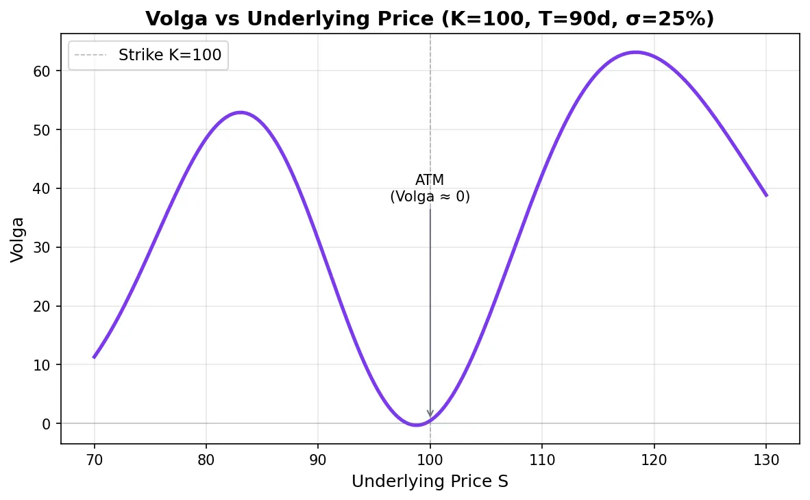
Volga’s distribution has a striking feature: ATM options have Volga near zero, while OTM options (especially deep wings) have large Volga.
Why? ATM options have \(d_1 \approx 0\) and \(d_2 \approx 0\), so \(d_1 \times d_2 \approx 0\), giving Volga ≈ 0. ATM options’ Vega responds almost linearly to IV: a 5-point IV move and a 10-point IV move produce nearly proportional Vega-driven P&L.
OTM options behave differently. Their \(|d_1|\) and \(|d_2|\) are both large, producing substantial Volga. When IV rises, OTM options’ Vega itself increases (because higher IV makes OTM options “closer” to ATM in probability space), so a large IV spike produces option price gains well above linear Vega estimates.
This directly explains a classic market phenomenon: why OTM options (especially OTM puts) are expensive. Beyond directional skew factors, Volga is the structural reason. Holding OTM puts means owning “volatility of volatility”; if markets panic (VIX from 15 to 40), OTM put gains far exceed linear Vega predictions because Volga amplifies the payoff. Market makers who sell OTM puts know this and charge Volga premium to compensate for the convexity risk.
Second-Order Greeks Interaction Matrix
First-order and second-order Greeks form a clean partial derivative network. Rows are the first-order quantity being differentiated; columns are the differentiation direction:
| w.r.t. \(S\) | w.r.t. \(\sigma\) | w.r.t. \(T\) | |
|---|---|---|---|
| Delta (\(\frac{\partial V}{\partial S}\)) | Gamma (\(\frac{\partial^2 V}{\partial S^2}\)) | Vanna (\(\frac{\partial^2 V}{\partial S \partial \sigma}\)) | Charm (\(\frac{\partial^2 V}{\partial S \partial T}\)) |
| Vega (\(\frac{\partial V}{\partial \sigma}\)) | Vanna (\(\frac{\partial^2 V}{\partial \sigma \partial S}\)) | Volga (\(\frac{\partial^2 V}{\partial \sigma^2}\)) | Veta (\(\frac{\partial^2 V}{\partial \sigma \partial T}\)) |
| Theta (\(\frac{\partial V}{\partial T}\)) | Charm (\(\frac{\partial^2 V}{\partial T \partial S}\)) | Veta (\(\frac{\partial^2 V}{\partial T \partial \sigma}\)) | — |
The symmetry is immediate: the matrix is symmetric about the diagonal (Schwarz’s theorem). Vanna appears twice, Charm appears twice, Veta appears twice. You do not need to memorize all cross-derivatives; the symmetry carries you.
Call/Put differences: Gamma, Vanna, and Volga are identical for calls and puts (same logic as first-order Gamma and Vega, since Put-Call Parity’s right side \(S - Ke^{-rT}\) has zero higher-order derivatives w.r.t. these variables). Charm differs between calls and puts because the mixed partial of \(S - Ke^{-rT}\) with respect to \(S\) and \(T\) is nonzero.
Volatility Surface and Second-Order Greeks
BSM assumes a single constant volatility \(\sigma\) across all strikes and expiries. One glance at an options chain disproves this: OTM put IV exceeds ATM IV, forming a volatility smile or skew.
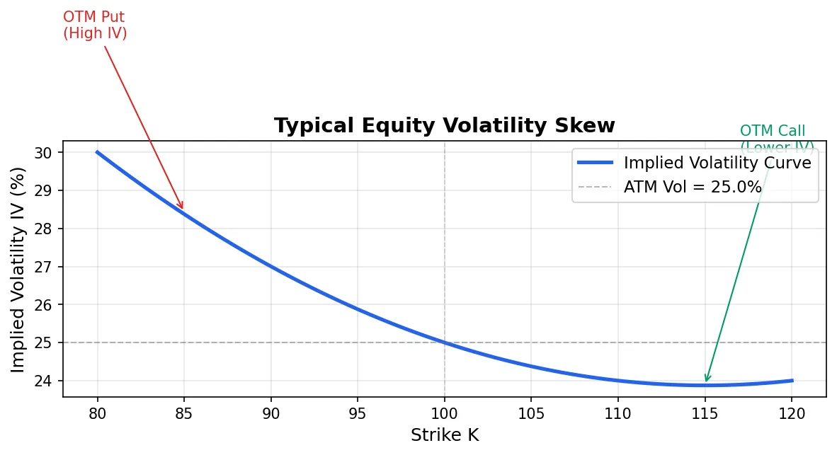
Why do smile and skew exist? The fundamental reason is that real asset returns are not normally distributed; they have fat tails and negative skew. The market prices OTM puts at higher IV to compensate for tail risk. From a pricing mechanics perspective, Vanna and Volga are the two core drivers of vol surface shape.
Vanna-Volga pricing is a practical correction to BSM. The idea is clean: price ATM options with BSM (which is accurate near ATM), then adjust with Vanna and Volga to add back the smile effect.
$$V_{VV} = V_{BSM} + \text{Vanna} \times \Delta\sigma_{skew} + \frac{1}{2} \text{Volga} \times (\Delta\sigma)^2$$This is not a rigorous derivation; it is a first/second-order Taylor expansion approximation. But in FX options markets, Vanna-Volga pricing has been the standard approach for decades, because FX vol surfaces are relatively flat and the second-order approximation is sufficiently accurate.
def vanna_volga_adjustment(S, K, T, r, sigma_atm, sigma_k, bsm2):
    """
    Vanna-Volga pricing adjustment (simplified)
    sigma_atm: ATM implied volatility
    sigma_k: market implied volatility at strike K
    bsm2: BSMSecondOrder instance (initialized with sigma_atm)
    """
    delta_sigma = sigma_k - sigma_atm
    vanna_adj = bsm2.vanna() * delta_sigma
    volga_adj = 0.5 * bsm2.volga() * delta_sigma**2
    return vanna_adj + volga_adj

# Example: ATM vol=25%, OTM Put (K=90) market vol=30%
bsm2_k90 = BSMSecondOrder(S=100, K=90, T=0.25, r=0.05, sigma=0.25)
adj = vanna_volga_adjustment(100, 90, 0.25, 0.05, 0.25, 0.30, bsm2_k90)
print(f"Vanna-Volga adjustment: {adj:.4f}")  # Positive: OTM Put priced above BSM
Sticky Strike vs. Sticky Delta: The vol surface has not only shape but dynamics. When the underlying moves from 100 to 105, the K=100 option goes from ATM to OTM. What happens to its IV?
- Sticky Strike: The K=100 IV does not change. The vol surface is “pinned” to strike levels. The underlying moved, so you moved along the moneyness axis. Most equity option markets approximate this behavior.
- Sticky Delta: Options at the same Delta level keep the same IV. The vol surface is “pinned” to Delta. The underlying moved, and the entire surface translated with it. Some FX markets approximate this behavior.
These two regimes require completely different Vanna hedging approaches. Under Sticky Strike, spot moves do not directly change IV, and Vanna’s impact works indirectly through Delta changes. Under Sticky Delta, spot moves are accompanied by IV changes, doubling Vanna exposure. Failing to distinguish between these regimes when hedging Vanna is a hidden source of P&L bleed in many quantitative strategies.
Next: Greeks Trading Applications
Second-order Greeks give you a finer-grained risk lens. Vanna lets you anticipate how IV changes impact your Delta hedge. Charm lets you pre-adjust for overnight drift. Volga explains why wings are structurally expensive.
But knowing the numbers is only the first step. How do you use them to build strategies, run dynamic hedges, and execute Gamma Scalping? The final article in this series: Option Greeks in Practice: Strategy Analysis, Hedging, and Gamma Scalping.
Series overview:
- Part 1: Option Greeks: Formulas, Python Code, and Charts
- Part 3: Option Greeks in Practice: Strategy Analysis, Hedging, and Gamma Scalping
- Tool: Option Greeks Calculator
For an overview of other quantitative trading metrics beyond options, see The Complete Guide to Quant Trading Metrics.