Options pricing is not about predicting direction. It is about quantifying multi-dimensional risk. The underlying price moves, time passes, volatility shifts, interest rates change, all simultaneously affecting an option’s value. Option Greeks extract the sensitivity of the option price to each of these variables, turning abstract risk into numbers you can hedge against.
This is part one of a three-part series on option Greeks, covering the five first-order Greeks (Delta, Gamma, Theta, Vega, Rho) with their mathematical formulas, intuitive explanations, and Python implementations. Parts two and three will cover second-order Greeks and trading applications, respectively.
Option Greeks at a Glance
Greeks are partial derivatives. The Black-Scholes model takes five inputs: spot price \(S\), strike price \(K\), time to expiry \(T\), risk-free rate \(r\), and volatility \(\sigma\). Differentiate the option price \(V\) with respect to each input, and you get the corresponding Greek.
| Greek | Symbol | Measures Sensitivity To | Call Range | Put Range |
|---|---|---|---|---|
| Delta | \(\Delta\) | $1 change in underlying price | [0, 1] | [-1, 0] |
| Gamma | \(\Gamma\) | Rate of change of Delta itself | > 0 | > 0 |
| Theta | \(\Theta\) | Daily time decay of option value | Usually < 0 | Usually < 0 |
| Vega | \(\mathcal{V}\) | 1% change in implied volatility | > 0 | > 0 |
| Rho | \(\rho\) | 1% change in interest rate | Call > 0 | Put < 0 |
Gamma and Vega are identical for calls and puts at the same strike and expiry. The proof is one step: put-call parity gives \(C - P = S - Ke^{-rT}\), and the right-hand side is linear in \(S\) and independent of \(\sigma\), so its second derivative w.r.t. \(S\) (Gamma) and derivative w.r.t. \(\sigma\) (Vega) are both zero. Theta can theoretically be positive (deep in-the-money puts), but in practice it is almost always negative.
The Black-Scholes Formula and the Mathematical Basis of Greeks
The BSM European call option pricing formula:
$$C = S \cdot N(d_1) - K e^{-rT} \cdot N(d_2)$$European put:
$$P = K e^{-rT} \cdot N(-d_2) - S \cdot N(-d_1)$$Where:
$$d_1 = \frac{\ln(S/K) + (r + \sigma^2/2)T}{\sigma\sqrt{T}}, \quad d_2 = d_1 - \sigma\sqrt{T}$$\(N(\cdot)\) is the standard normal CDF, and \(N'(\cdot)\) is the corresponding PDF.
The intuition behind \(d_1\): it measures how far the current spot price is from the strike, normalized by volatility-adjusted distance. The larger \(d_1\) is, the deeper in-the-money the option, and the more it behaves like holding the underlying directly. \(N(d_2)\) is the risk-neutral probability of expiring in-the-money; \(d_2\) is the corresponding standard normal quantile.
Here is a complete Python implementation that computes BSM prices and all first-order Greeks. Every analysis in the following sections builds on this code:
import numpy as np
from scipy.stats import norm
class BSMCalculator:
"""Black-Scholes-Merton option pricing and Greeks"""
def __init__(self, S, K, T, r, sigma):
"""
S: spot price
K: strike price
T: time to expiry (years)
r: risk-free rate
sigma: volatility
"""
self.S = S
self.K = K
self.T = T
self.r = r
self.sigma = sigma
self.d1 = (np.log(S / K) + (r + 0.5 * sigma**2) * T) / (sigma * np.sqrt(T))
self.d2 = self.d1 - sigma * np.sqrt(T)
def call_price(self):
return self.S * norm.cdf(self.d1) - self.K * np.exp(-self.r * self.T) * norm.cdf(self.d2)
def put_price(self):
return self.K * np.exp(-self.r * self.T) * norm.cdf(-self.d2) - self.S * norm.cdf(-self.d1)
def delta(self, option_type='call'):
if option_type == 'call':
return norm.cdf(self.d1)
return norm.cdf(self.d1) - 1
def gamma(self):
return norm.pdf(self.d1) / (self.S * self.sigma * np.sqrt(self.T))
def theta(self, option_type='call'):
"""Returns daily Theta (annualized value / 365)"""
common = -self.S * norm.pdf(self.d1) * self.sigma / (2 * np.sqrt(self.T))
if option_type == 'call':
return (common - self.r * self.K * np.exp(-self.r * self.T) * norm.cdf(self.d2)) / 365
return (common + self.r * self.K * np.exp(-self.r * self.T) * norm.cdf(-self.d2)) / 365
def vega(self):
"""Returns price change per 1% volatility move"""
return self.S * norm.pdf(self.d1) * np.sqrt(self.T) / 100
def rho(self, option_type='call'):
"""Returns price change per 1% interest rate move"""
if option_type == 'call':
return self.K * self.T * np.exp(-self.r * self.T) * norm.cdf(self.d2) / 100
return -self.K * self.T * np.exp(-self.r * self.T) * norm.cdf(-self.d2) / 100
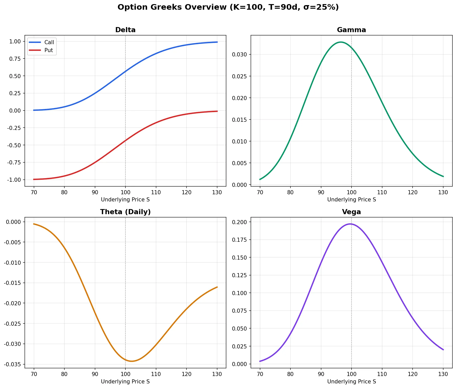
# Example: S=100, K=100, T=0.25 (90 days), r=5%, sigma=25%
bsm = BSMCalculator(S=100, K=100, T=0.25, r=0.05, sigma=0.25)
print(f"Call Price: {bsm.call_price():.4f}") # 5.5984
print(f"Put Price: {bsm.put_price():.4f}") # 4.3562
print(f"Call Delta: {bsm.delta('call'):.4f}") # 0.5645
print(f"Put Delta: {bsm.delta('put'):.4f}") # -0.4355
print(f"Gamma: {bsm.gamma():.4f}") # 0.0315
print(f"Call Theta: {bsm.theta('call'):.4f}") # -0.0339
print(f"Vega: {bsm.vega():.4f}") # 0.1969
print(f"Call Rho: {bsm.rho('call'):.4f}") # 0.1271
Two conventions trip people up regularly. Theta: some textbooks give annualized values, others give per-calendar-day, others per-trading-day (dividing by 252 instead of 365). Most brokers and trading platforms use calendar-day Theta (divided by 365), which is what the code above does. Vega: some define it as the price change for a 1.0 (i.e., 100 percentage points) volatility move, others for a 0.01 (1 percentage point) move, a factor of 100 difference. The code above uses the “1 percentage point” convention, matching market-maker quoting practice.
This code is for teaching purposes and has no input validation. \(T \leq 0\) or \(\sigma \leq 0\) will cause division by zero or NaN. Production code should add parameter sanity checks.
The chart below shows all five Greeks in a single view:
Delta: Price Sensitivity to the Underlying
Delta under BSM is straightforward:
$$\Delta_{call} = N(d_1), \quad \Delta_{put} = N(d_1) - 1$$Delta carries three layers of meaning, each useful in practice.
Price sensitivity. A call with Delta 0.5 means the option price moves roughly $0.50 for every $1 move in the underlying. “Roughly” because this is a linear approximation: Delta itself is changing (which is Gamma’s domain).
Hedge ratio. Holding one call contract (100 multiplier) with Delta 0.5 requires shorting 50 shares to build a delta-neutral position. Market makers spend their days doing exactly this: continuously adjusting their stock position to keep net portfolio Delta near zero.
Approximate expiry probability. Delta’s absolute value loosely represents the probability of expiring in-the-money. A 0.3-Delta call has roughly a 30% chance of finishing ITM. This is not the exact probability (that would be \(N(d_2)\), not \(N(d_1)\)), but it is close enough for quick assessment.
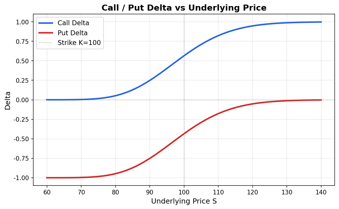
The S-shaped curve tells the story: deep OTM calls have Delta near 0, deep ITM calls approach 1. Around the ATM strike, Delta sits near 0.5 and changes fastest, meaning ATM options demand the most frequent hedging.
Hedge frequency is a real operational decision. BSM assumes continuous rehedging (infinite frequency), but every hedge trade incurs transaction costs. Hedge too often and costs eat your profits; too infrequently and Gamma exposure becomes dangerously large. Most market makers use a Delta bandwidth approach: rehedge only when net Delta exceeds a threshold (e.g., ±200 share equivalents), rather than adjusting every minute. The optimal bandwidth depends on Gamma magnitude and transaction costs; there is no one-size-fits-all answer.
Gamma: The Rate of Change of Delta
Gamma is the second partial derivative of option price with respect to the underlying:
$$\Gamma = \frac{N'(d_1)}{S \cdot \sigma \cdot \sqrt{T}}$$where \(N'(d_1)\) is the standard normal PDF evaluated at \(d_1\).
Gamma is always positive (identical for calls and puts). It peaks at ATM and decays rapidly on either side. The intuition: ATM options are where Delta is transitioning from 0 toward 1 (or -1 toward 0) most aggressively. Deep ITM or OTM options have nearly static Deltas, so their Gamma is negligible.
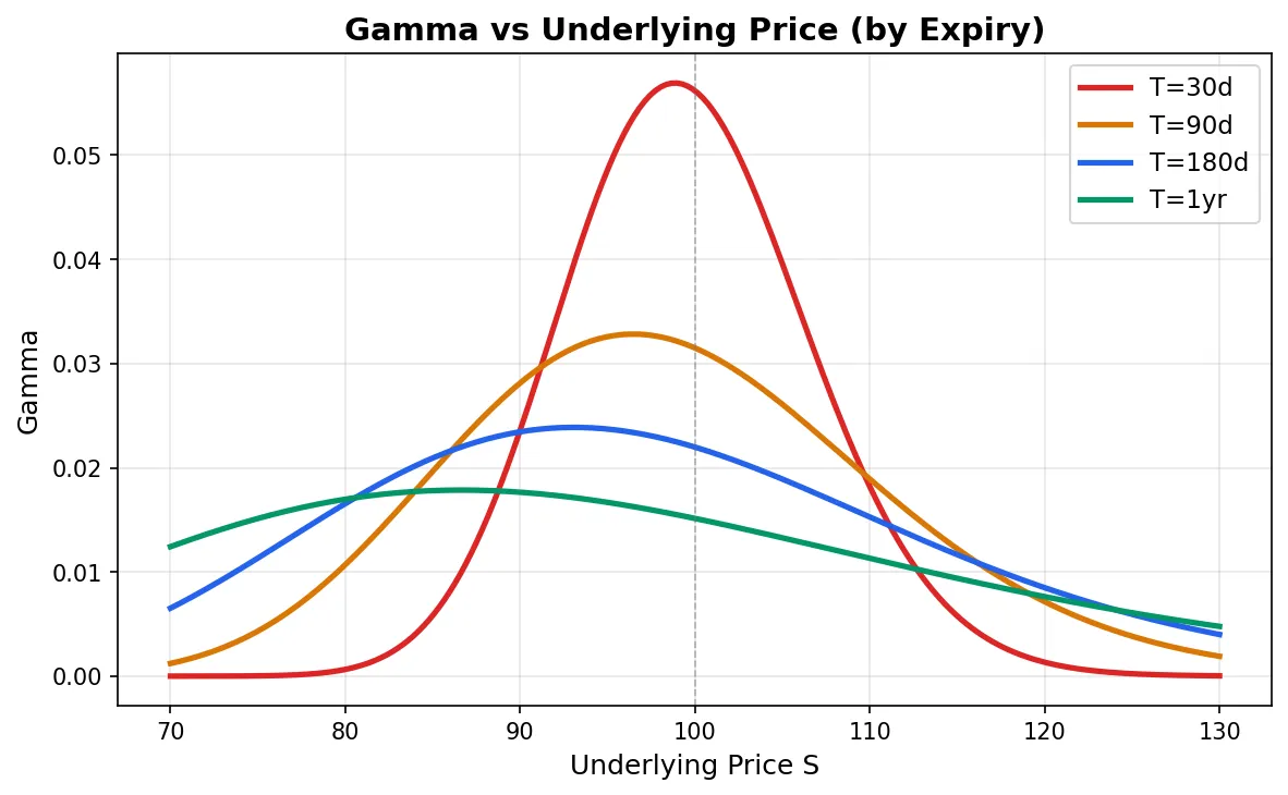
A critical observation from the chart: shorter-dated options have dramatically higher ATM Gamma but a much narrower Gamma curve. An ATM option with two days to expiry can see its Delta swing from 0.3 to 0.7 on a modest move in the underlying. This is Gamma risk, and it is the reason market makers get visibly nervous in the last day or two before expiration.
Long Gamma vs. Short Gamma:
- Long Gamma (option buyers): The underlying can move in either direction and you benefit. Rally: you make more than a linear estimate. Drop: you lose less. The numerical example below spells out the math. The cost is that Theta bleeds your account every morning.
- Short Gamma (option sellers): You collect Theta every day, until the underlying gaps 5% and Gamma hands back everything you earned, plus extra. The February 2018 VIX blowup was Short Gamma taken to its logical extreme.
A numerical example of Long Gamma’s convexity benefit (using rounded Delta=0.50, Gamma=0.03 for clean arithmetic, not the exact values from the code above): you hold an ATM call with Gamma = 0.03 and Delta = 0.50. The underlying rallies from 100 to 105. Your Delta becomes approximately 0.65 (= 0.50 + 0.03 × 5). Your profit is not the linear estimate of 0.50 × 5 = 2.50, but approximately (0.50 + 0.65)/2 × 5 = 2.875. The extra 0.375 is Gamma’s convexity benefit. If the underlying drops 5 instead, your loss is about (0.50 + 0.35)/2 × 5 = 2.125, less than the linear estimate of 2.50. You gain more on up moves and lose less on down moves. The catch: Theta erodes your position every day. Note that the linear Gamma approximation (\(\Delta_{new} = \Delta + \Gamma \cdot \Delta S\)) is only accurate for small moves; for large moves, Gamma itself changes, and actual Delta will deviate from the linear estimate.
Theta: Time Works Against Option Buyers
The call Theta formula:
$$\Theta_{call} = -\frac{S \cdot N'(d_1) \cdot \sigma}{2\sqrt{T}} - r \cdot K \cdot e^{-rT} \cdot N(d_2)$$Theta is almost always negative from the buyer’s perspective: option value erodes as time passes. ATM options have the largest absolute Theta because they carry the most time value and therefore the most to lose.
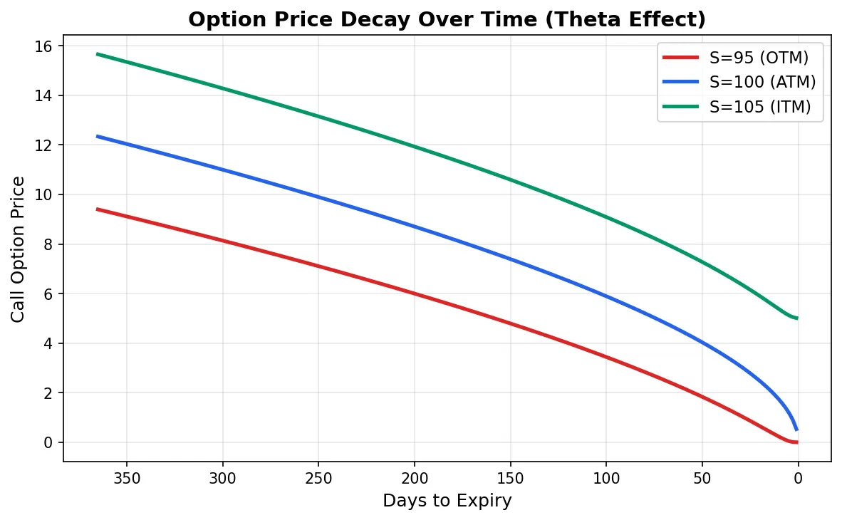
The most important feature of this chart: decay is nonlinear and accelerates sharply in the final 30 days. The ATM option (blue line) barely loses value in the first six months, then drops precipitously in the last month. This directly shapes strategy choice:
- Sellers (covered calls, iron condors) prefer selling short-dated options because Theta harvesting is most efficient in the final 30 days
- Buyers should avoid holding into the last month unless positioned for a specific directional event (earnings, FDA decisions)
Theta and Gamma sit on opposite ends of a seesaw. Under BSM, for a delta-neutral portfolio:
$$\Theta + \frac{1}{2} \sigma^2 S^2 \Gamma = r \cdot V$$When \(r \approx 0\), this simplifies to \(\Theta \approx -\frac{1}{2} \sigma^2 S^2 \Gamma\). Long Gamma costs you negative Theta. Short Gamma rewards you with positive Theta. You cannot hold positive Gamma and positive Theta simultaneously; risk and reward must balance. When you build a spread and the Gamma-Theta ratio looks off, this equation is the first thing to check.
Vega: What a One-Point Vol Move Is Worth
$$\mathcal{V} = S \cdot N'(d_1) \cdot \sqrt{T}$$The formula above gives Vega for a 1.0 (100 percentage points) volatility change. In practice, divide by 100 to get the price impact of a 1 percentage point volatility move, e.g., volatility shifting from 25% to 26%.
Like Gamma, Vega peaks at ATM. But Vega has the opposite relationship with time: longer-dated options have larger Vega. A one-year ATM option is far more sensitive to volatility than a one-month ATM option, because volatility has a longer runway to compound.
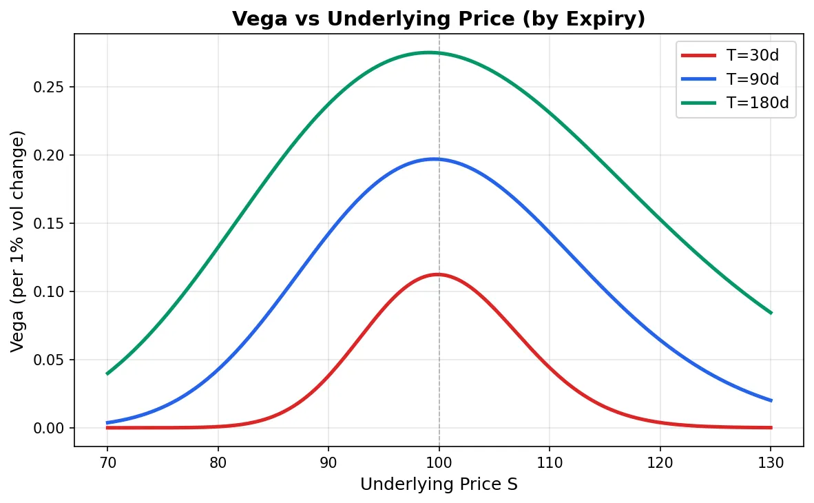
IV Crush is Vega’s most visible real-world manifestation. Before a company reports earnings, implied volatility (IV) typically gets bid up to 50%, 60%, or higher as the market prices in the expected post-earnings move. After the report, uncertainty resolves, and IV collapses back to normal levels, perhaps from 60% down to 30%. If you are holding an ATM call with Vega = 0.20, that 30-point IV drop alone costs you 0.20 × 30 = $6.00. Even if the stock moves in your predicted direction, the Delta gains may not cover the Vega losses from IV Crush. This is why many traders buy options before earnings, get the direction right, and still lose money. Vega is the real killer.
Rho: Interest Rate Sensitivity
$$\rho_{call} = K \cdot T \cdot e^{-rT} \cdot N(d_2), \quad \rho_{put} = -K \cdot T \cdot e^{-rT} \cdot N(-d_2)$$Rho is safely ignored in most scenarios. For short-term options (1-3 months), a 25 basis point rate change moves the option price by pennies. Two exceptions:
Long-dated options (LEAPS) with 1-2 years to expiry can have Rho above 0.50, meaning a 1% rate move shifts the option price by $0.50. During the 2022-2023 Fed hiking cycle, LEAPS pricing was noticeably affected.
Rapid rate-change environments. If a central bank hikes 200-300 basis points over several months, even medium-term options accumulate material Rho impact.
Next: Second-Order Greeks and the Volatility Surface
With Delta, Gamma, Theta, and Vega, you can answer the four questions that matter for any options position: how much do I make if the stock moves a dollar? What if it moves five? What does holding overnight cost me? And what happens when IV drops 10 points?
But first-order descriptions are incomplete. Delta itself changes with volatility (that is Vanna) and with time (that is Charm). Vega has its own convexity (Volga). Market makers running large options books must monitor second-order Greeks to avoid blind spots. The next article in this series covers these higher-order sensitivities and their role in volatility surface modeling.
Series navigation:
- Part 2: Second-Order Greeks: Vanna, Charm, Volga and Volatility Surfaces
- Part 3: Option Greeks in Practice: Strategy Analysis, Hedging, and Gamma Scalping
- Tool: Option Greeks Calculator
For an overview of other quantitative trading metrics beyond options, see The Complete Guide to Quant Trading Metrics.