The same strategy at 10% position size and 50% position size can mean the difference between steady compounding and a blown account. Stock selection, timing, and factor design answer “what to buy.” Position sizing answers “how much.” The Kelly Criterion is the mathematical optimum for that question.
The Classic Kelly Formula
The Kelly Criterion comes from John Kelly at Bell Labs in 1956. The original setting is a simple binary gamble: win probability \(p\), loss probability \(q = 1-p\), payout odds \(b\) (win returns \(b\) times your wager, loss takes the entire wager). You have a bankroll. What fraction do you bet each round?
Kelly’s answer:
$$f^* = \frac{bp - q}{b} = \frac{bp - (1-p)}{b}$$where \(f^*\) is the optimal bet fraction (percentage of total capital).
Numerical example: win rate 55%, odds 1:1 (\(b=1\)).
$$f^* = \frac{1 \times 0.55 - 0.45}{1} = 0.10$$The optimal bet is 10% of your bankroll. Intuition checks out: you have a slight edge but should not bet big.
Kelly maximizes not the expected profit per round, but the expected logarithmic growth rate of wealth. Log growth is the engine of geometric compounding. Arithmetic expectation can be high, but a single total loss sends the geometric growth rate to negative infinity. Kelly finds the \(f\) that maximizes \(E[\ln(W)]\), where \(W\) is post-round wealth.
The derivation: after each round, wealth is \(W_{n+1} = W_n(1 + f \cdot X)\), where \(X\) is \(+b\) (probability \(p\)) or \(-1\) (probability \(q\)). The expected log growth rate:
$$G(f) = p \ln(1 + bf) + q \ln(1 - f)$$Take the derivative with respect to \(f\), set it to zero, and the formula above drops out.
An important property: \(f^*\) is positive only when the expected value is positive. If \(bp < q\) (negative expectation), the formula returns a negative number, meaning you should not bet (or should bet the other side). No edge, no bet.
Continuous Case: Kelly for Return Distributions
Real trading returns are not binary. Asset returns follow continuous distributions. Assuming log-normal returns with mean \(\mu\), standard deviation \(\sigma\), and risk-free rate \(r\), the continuous Kelly formula is:
$$f^* = \frac{\mu - r}{\sigma^2}$$Intuition: \(\mu - r\) is excess return (your edge), \(\sigma^2\) is risk (variance). More edge means larger position; more risk means smaller position.
The connection to the Sharpe ratio is direct. Sharpe ratio \(SR = \frac{\mu - r}{\sigma}\), so:
$$f^* = \frac{SR}{\sigma}$$A strategy with Sharpe 1.0 and annualized volatility 20% has an optimal Kelly leverage of \(1.0 / 0.20 = 5\times\). Sharpe 0.5, volatility 30%: Kelly leverage is \(0.5 / 0.30 \approx 1.67\times\).
This reveals something important: many quant strategies have Kelly-optimal leverage far higher than intuition suggests. A strategy with 15% annual return, 10% volatility (\(\mu - r = 0.10\), assuming \(r = 5\%\)) has Kelly leverage of \(0.10 / 0.01 = 10\times\). Running 10x leverage is theoretically growth-maximizing, but the ride will be brutal.
Fractional Kelly: The Practical Key
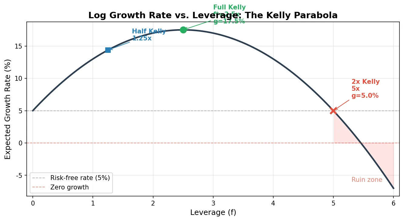
Using the raw \(f^*\) from the formula as your position size is called full Kelly. In the previous section’s example, \(f^* = 2.5\) means full Kelly demands 2.5x leverage. Full Kelly maximizes the theoretical growth rate, but has serious practical problems:
- Deep drawdowns. Full Kelly’s theoretical maximum drawdown can approach 100%. In simulations of 1000 bets, full Kelly routinely sees 50-80% drawdowns along the path.
- Parameter estimation error gets amplified. You estimate \(\mu\) and \(\sigma\) from historical data, but these are just estimates. If the true \(\mu\) is lower than your estimate, full Kelly becomes an over-bet, and the consequences are catastrophic. Over-betting is far more dangerous than under-betting: under-bet just grows slower; over-bet past a threshold and long-run growth rate turns negative.
So in practice, nearly everyone uses fractional Kelly: instead of using \(f^*\) directly, multiply it by a factor less than 1. \(f^*/2\) is called half Kelly, \(f^*/3\) is one-third Kelly. If full Kelly is 2.5x leverage, half Kelly is 1.25x, one-third Kelly is 0.83x.
Half Kelly has attractive properties:
- Expected growth rate is 75% of full Kelly (only 25% growth speed sacrificed)
- Maximum drawdown roughly halved
- Much more robust to parameter estimation error
Python simulation comparing full Kelly, half Kelly, and fixed position sizing:
import numpy as np

def simulate_kelly(mu, sigma, r, fraction, n_days=1000, n_sims=500):
    """
    Simulate wealth paths under different Kelly fractions
    mu: annualized strategy return
    sigma: annualized strategy volatility
    fraction: Kelly fraction (1.0=full, 0.5=half)
    """
    dt = 1 / 252  # daily
    kelly_full = (mu - r) / sigma**2
    f = kelly_full * fraction

    daily_mu = mu * dt
    daily_sigma = sigma * np.sqrt(dt)

    np.random.seed(42)
    returns = np.random.normal(daily_mu, daily_sigma, (n_sims, n_days))

    # Daily: Kelly fraction in strategy, rest in risk-free
    wealth = np.ones((n_sims, n_days + 1))
    for t in range(n_days):
        portfolio_return = f * returns[:, t] + (1 - f) * r * dt
        wealth[:, t + 1] = wealth[:, t] * (1 + portfolio_return)

    return wealth

mu, sigma, r = 0.15, 0.20, 0.05

wealth_full = simulate_kelly(mu, sigma, r, fraction=1.0)
wealth_half = simulate_kelly(mu, sigma, r, fraction=0.5)
wealth_fixed = simulate_kelly(mu, sigma, r, fraction=0.3)  # fixed 30%

for name, w in [("Full Kelly", wealth_full), ("Half Kelly", wealth_half), ("Fixed 30%", wealth_fixed)]:
    final = w[:, -1]
    median_return = np.median(final)
    max_dd = np.min(w / np.maximum.accumulate(w, axis=1), axis=1)
    avg_max_dd = np.mean(1 - max_dd)
    print(f"{name}: median final={median_return:.2f}, avg max drawdown={avg_max_dd:.1%}")
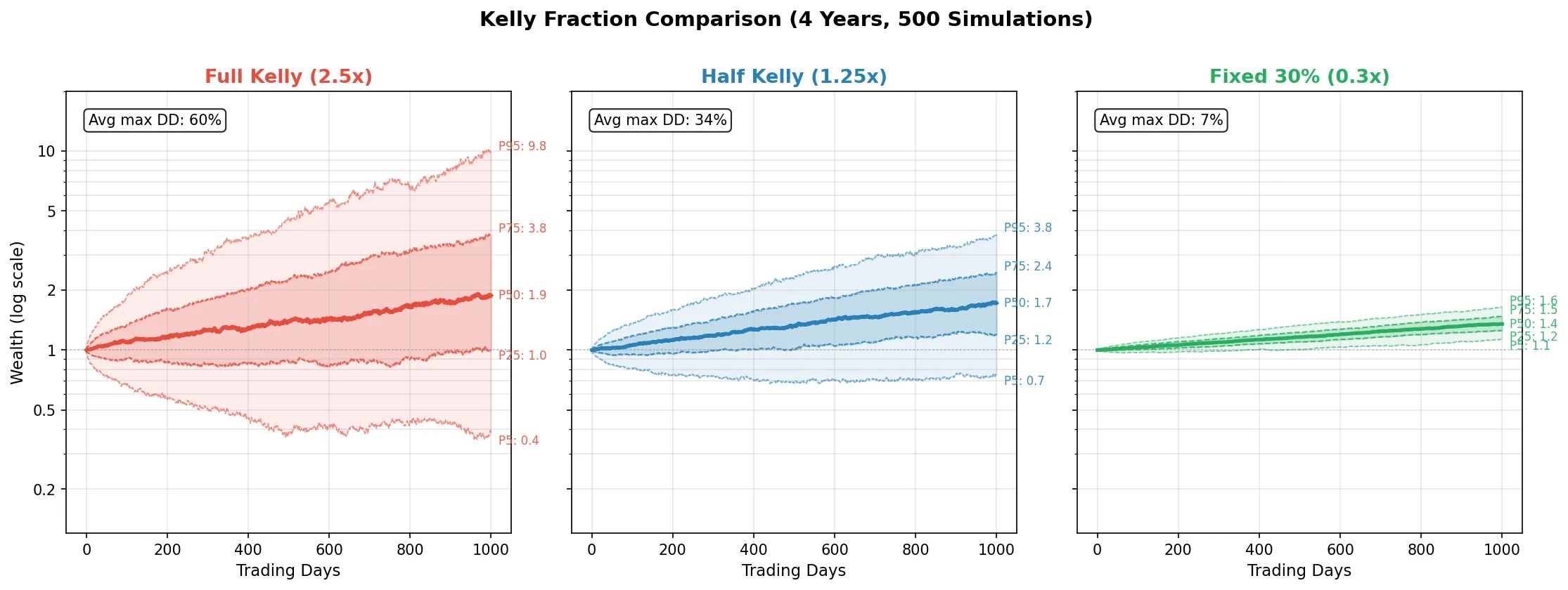
Parameters: annualized return \(\mu=15\%\), volatility \(\sigma=20\%\), risk-free rate \(r=5\%\). First compute the full Kelly optimal leverage: \(f^* = (0.15 - 0.05) / 0.20^2 = 2.5\), meaning the formula says to put 250% of your capital into the strategy (2.5x leverage). Full Kelly (fraction=1.0) uses that 2.5x directly; half Kelly (fraction=0.5) takes half, i.e., 1.25x; fixed 30% ignores the formula and always invests 30% of capital. 500 paths, 1000 trading days each (about 4 years). Results:
| Leverage | Median Final | Mean Final | Avg Max DD | 95th Pct Max DD | |
|---|---|---|---|---|---|
| Full Kelly | 2.50x | 1.88 | 3.13 | 60.3% | 81.9% |
| Half Kelly | 1.25x | 1.72 | 1.96 | 34.5% | 52.4% |
| Fixed 30% | 0.30x | 1.54 | 1.62 | 20.9% | 32.9% |
The pattern is clear: full Kelly at 2.5x leverage has the highest median terminal wealth (1.88 vs 1.72), but the cost is a 60% average max drawdown, with the 95th percentile reaching 82%. Half Kelly uses only 1.25x leverage, terminal wealth is just 8% lower, while drawdown is nearly halved. Fixed 30% is the most conservative at 21% drawdown. Note that mean terminal wealth (3.13) is far above median (1.88), indicating full Kelly’s distribution is heavily right-skewed: a few paths compound spectacularly and pull up the mean, but most paths do not perform as well as the mean suggests.
Multi-Asset Kelly
Single-asset Kelly needs one ratio. Multiple assets require the covariance matrix. Given \(n\) assets with return vector \(\boldsymbol{\mu}\), covariance matrix \(\boldsymbol{\Sigma}\), and risk-free rate \(r\), the multi-asset Kelly optimal weight vector is:
$$\mathbf{f}^* = \boldsymbol{\Sigma}^{-1} (\boldsymbol{\mu} - r \cdot \mathbf{1})$$This connects directly to mean-variance optimization (Markowitz). The Markowitz tangency portfolio (maximum Sharpe ratio portfolio) has weights proportional to \(\boldsymbol{\Sigma}^{-1}(\boldsymbol{\mu} - r \cdot \mathbf{1})\), but normalized to a target risk level. The Kelly portfolio is the tangency portfolio without normalization, using whatever leverage falls out of the math.
In practice, nobody uses this formula raw, because \(\boldsymbol{\Sigma}^{-1}\) is highly unstable in high dimensions (large condition number; small perturbations cause wild weight swings). Common workarounds:
- Use a shrinkage estimator (e.g., Ledoit-Wolf) to regularize the covariance matrix
- Add weight constraints (e.g., no single asset above 20%)
- Multiply by a fractional Kelly factor (e.g., 1/3) to reduce overall leverage
If you are doing position sizing for a factor portfolio, multi-asset Kelly provides the theoretical framework: each factor’s weight should be proportional to its excess return divided by its contribution to portfolio variance.
import numpy as np

def multi_asset_kelly(mu, cov, r, fraction=0.5):
    """
    Multi-asset Kelly weights
    mu: (n,) expected annualized returns
    cov: (n, n) return covariance matrix
    r: risk-free rate
    fraction: Kelly fraction
    """
    excess = mu - r
    cov_inv = np.linalg.inv(cov)
    kelly_weights = cov_inv @ excess * fraction
    return kelly_weights

# Example: 3 assets
mu = np.array([0.12, 0.08, 0.15])    # annualized returns
sigma = np.array([0.20, 0.15, 0.25]) # annualized volatilities
corr = np.array([
    [1.0, 0.3, 0.5],
    [0.3, 1.0, 0.2],
    [0.5, 0.2, 1.0]
])
cov = np.outer(sigma, sigma) * corr
r = 0.05

weights = multi_asset_kelly(mu, cov, r, fraction=0.5)
print("Half Kelly weights:", np.round(weights, 3))
print("Total leverage:", round(np.sum(np.abs(weights)), 2))
Output:
Half Kelly weights: [0.441 0.294 0.588]
Total leverage: 1.32
Asset 3 (excess return 10%, volatility 25%) gets the highest weight at 0.588, despite having the highest volatility, because its excess return is also the highest. Asset 2 (excess return 3%, volatility 15%) gets the lowest weight. Total leverage is 1.32x, much milder than single-asset Kelly, because correlations between assets diversify risk (the covariance matrix inverse implicitly accounts for diversification).
Practical Considerations
Parameter estimation error is the biggest enemy. Kelly assumes you know the true \(\mu\) and \(\sigma\). In reality, you only have sample estimates. \(\mu\) estimation is especially unreliable: with 250 trading days, the standard error of \(\mu\) is approximately \(\sigma / \sqrt{250} \approx \sigma / 16\). For a strategy with 20% annual volatility, the standard error of \(\mu\) is 1.25%. If you estimate \(\mu = 15\%\), the true value might be anywhere from 12% to 18%. Plug these into Kelly and the optimal position size can differ by a factor of two.
This connects directly to backtesting pitfalls. If you overfit parameters in backtesting, \(\mu\) gets inflated, Kelly gives you an oversized position, and live trading blows up.
Never exceed the Kelly position. The Kelly fraction is the boundary where growth rate peaks: at full Kelly, growth is maximized; above full Kelly, growth rate declines; above 2x Kelly, growth rate turns negative (guaranteed long-run loss). Under-betting just slows growth. Over-betting past a threshold guarantees long-run ruin. The asymmetry is stark.
Subtract transaction costs from returns. Kelly assumes frictionless markets. If the strategy requires frequent rebalancing, transaction costs (commissions, slippage, market impact) eat into \(\mu\). Use \(\mu_{\text{net}} = \mu - \text{costs}\) in the Kelly formula and the position shrinks. This adjustment matters most for high-frequency strategies.
Short volatility is especially dangerous. As discussed in volatility trading strategies, selling volatility produces negatively skewed returns (small gains most of the time, occasional large losses). Kelly under the normal assumption systematically overestimates the optimal position for negatively skewed distributions. The Kelly position for selling VIX futures under normal assumptions versus the true fat-tailed distribution can differ dramatically. This is one of the structural reasons short-vol funds blew up in February 2018.
Kelly is a ceiling, not a target. In practice, most quantitative funds use 1/4 to 1/2 Kelly. The tradeoff: give up some growth speed in exchange for manageable drawdowns and robustness to estimation error. If you are unsure how much to use, half Kelly is a reasonable starting point.