Gamma scalping is a core strategy for market makers and volatility traders. The logic is straightforward: buy a straddle to establish positive Gamma exposure, then continuously delta-hedge to convert the underlying’s price oscillations into locked-in profits. You are not betting on direction. You are betting that realized volatility will exceed the implied volatility you paid for.
This is the exact opposite of selling volatility. Short-vol traders want the underlying to stay still and collect Theta decay. Gamma scalpers want the underlying to move aggressively, generating enough hedge profits to more than cover the daily time decay.
What Gamma Scalping Actually Earns
After buying an ATM straddle, you hold a positive Gamma position. Gamma causes your Delta to shift favorably as the underlying moves: when the stock rises, your net Delta becomes positive (you are automatically getting long); when it falls, your Delta becomes negative (you are automatically getting short).
This convexity means large moves help you disproportionately. A $2 move generates more than twice the profit of a $1 move.
Gamma scalping mechanically “flattens” this auto-generated Delta: stock goes up, you sell shares to push Delta back to zero; stock goes down, you buy shares. Each hedge is a “sell high, buy low” transaction. As long as the underlying keeps oscillating, you keep locking in small gains.
The cost is Theta decay. Your options lose value every day. If the stock barely moves, the hedge profits are negligible compared to what Theta takes from you.
The core bet: realized volatility will exceed implied volatility. You paid for IV when buying the options. You “collect” RV through hedging. If RV > IV, you profit. If RV < IV, you lose.
The Math: Gamma P&L vs Theta P&L
This section builds intuition for why enough movement makes money and too little movement loses.
For a delta-neutral options portfolio, the P&L over a small time interval \(\Delta t\) approximates to:
$$\text{P\&L} \approx \frac{1}{2} \Gamma (\Delta S)^2 + \Theta \cdot \Delta t$$The first term is Gamma P&L: the convexity gain from the underlying moving \(\Delta S\). It is proportional to \((\Delta S)^2\) and always positive for long gamma. The second term is Theta P&L: the time decay cost, always negative when you own options.
Breakeven condition:
$$\frac{1}{2} \Gamma (\Delta S)^2 + \Theta \cdot \Delta t = 0$$Solving for the minimum daily move:
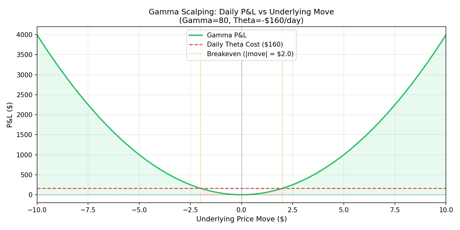
$$|\Delta S|_{\text{breakeven}} = \sqrt{\frac{-2\Theta}{\Gamma}}$$Concrete example: your portfolio has Gamma = 80 (10 straddles) and daily Theta = -$160.
$$|\Delta S|_{\text{breakeven}} = \sqrt{\frac{2 \times 160}{80}} = \sqrt{4} = 2$$The underlying must move at least $2 per day to break even. Moves larger than $2 generate profit; smaller moves result in losses.
Converting to annualized volatility: if the underlying is at $500, a daily $2 move corresponds to roughly:
$$\sigma_{\text{breakeven}} = \frac{2}{500} \times \sqrt{252} \approx 6.3\%$$If you bought the straddle at 18% IV, you need realized volatility above 18% to profit. This aligns with the intuition: you paid for 18% IV, so the market needs to deliver at least 18% RV.
Step-by-Step: A Complete Gamma Scalping Example
Opening the Position
Underlying: SPY at $502 Buy: 10 contracts of 30-day ATM straddle ($502 strike) Cost: Call $7.80 + Put $7.40 = $15.20 per contract, total $15,200
Initial Greeks (10 contracts combined):
- Delta: roughly +20 (near zero)
- Gamma: +80
- Theta: -$160/day
- Vega: +$440
Sell 20 shares to flatten the initial Delta to zero.
Day 1: SPY Rallies to $504
The stock moves up $2. New Delta ≈ 20 + 80 × 2 = +180. You are now effectively long 180 shares.
Action: sell 180 shares of SPY at $504. Delta returns to zero.
Day 2: SPY Drops to $501
The stock drops $3. Delta ≈ 0 + 80 × (-3) = -240.
Action: buy 240 shares of SPY at $501.
From a hedging perspective: you sold 180 shares at $504 on Day 1, and bought 240 shares at $501 on Day 2. Of those, 180 shares form a complete round-trip, earning $3 per share = $540.
Two days of Theta: $160 × 2 = $320.
Net P&L: $540 - $320 = +$220. Realized volatility was large enough. Gamma scalping wins.
Day 3: SPY Moves Only $0.50
Delta change = 80 × 0.5 = 40. Hedging 40 shares captures roughly $0.50 × 40 / 2 = $10.
Theta cost: $160.
Net P&L: -$150. The stock did not move enough. Theta eats the position alive.
This is the daily rhythm of gamma scalping: big-move days accumulate profits, quiet days bleed. The final outcome depends on whether cumulative realized volatility over the holding period exceeds the implied volatility at entry.
Hedge Frequency: How Often to Rebalance
This is a critical operational decision. Hedging too frequently (every $0.10 move) racks up transaction costs. Hedging too rarely (once a day) risks letting intraday moves reverse before you capture them.
Three common approaches:
Fixed time intervals. Hedge at close, or every 4 hours. Simple to manage but sluggish on volatile days.
Fixed Delta threshold. Trigger a hedge when Delta drifts beyond a set value (e.g., ±50 shares). More adaptive, but trade count is unpredictable.
Fixed percentage move. Hedge each time the underlying moves 1%. A compromise that most market makers use in some form.
For 30-day ATM straddles, retail traders generally find the fixed-threshold approach practical (hedge when Delta exceeds Gamma × 1% of underlying price). This produces roughly 2-4 hedges per day with manageable transaction costs.
Gamma Scalping vs Theta Selling
| Dimension | Gamma Scalping | Theta Selling (Short Straddle / Iron Condor) |
|---|---|---|
| Core Greek | Long Gamma | Positive Theta |
| Market assumption | Large moves expected | Range-bound / quiet market |
| Profit source | RV > IV | IV > RV |
| Daily experience | Bleeding most days, occasional big wins | Collecting most days, occasional big losses |
| Activity level | High, frequent hedging | Low, open and wait |
| Primary risk | No movement, Theta burns the options | Large move, Gamma amplifies losses |
| Capital efficiency | Lower, must pay for options | Higher, collects premium upfront |
The two strategies are mirror images. Most of the time markets are mean-reverting and short vol wins. But around trend moves and high-impact events (earnings, FOMC, black swans), gamma scalping outperforms.
Many experienced options traders run both: a theta portfolio in normal conditions, plus small gamma scalp positions around specific event windows as a hedge.
Python Simulation: Gamma Scalping P&L Under Different Volatility Regimes
The code below simulates random walks of the underlying at different realized volatility levels and computes gamma scalping P&L. It helps visualize exactly how much RV you need to profit.
import numpy as np
import matplotlib.pyplot as plt

def simulate_gamma_scalp(
    S0=500, RV=0.25, T=30,
    gamma_per_dollar=0.16, theta_per_day=-160,
    n_simulations=1000
):
    """
    Simulate gamma scalping P&L under a given realized volatility.
    Simplified: assumes constant Gamma and Theta throughout.
    """
    daily_vol = RV / np.sqrt(252)
    pnl_list = []
    for _ in range(n_simulations):
        price = S0
        cumulative_hedge_pnl = 0.0
        for day in range(T):
            daily_return = np.random.normal(0, daily_vol)
            move = price * daily_return
            price += move
            cumulative_hedge_pnl += 0.5 * gamma_per_dollar * move**2
        total_pnl = cumulative_hedge_pnl + theta_per_day * T
        pnl_list.append(total_pnl)
    return np.array(pnl_list)

# Simulate across different RV levels
rv_levels = [0.12, 0.16, 0.20, 0.24, 0.28, 0.32]
results = {rv: simulate_gamma_scalp(RV=rv) for rv in rv_levels}

# --- Visualization ---
fig, axes = plt.subplots(1, 2, figsize=(14, 5))

mean_pnls = [results[rv].mean() for rv in rv_levels]
colors = ["#ef4444" if m < 0 else "#22c55e" for m in mean_pnls]
axes[0].bar([f"{int(rv*100)}%" for rv in rv_levels], mean_pnls, color=colors)
axes[0].axhline(y=0, color="#6b7280", linewidth=0.8)
axes[0].set_xlabel("Realized Volatility", fontsize=11)
axes[0].set_ylabel("Average P&L ($)", fontsize=11)
axes[0].set_title("Gamma Scalping P&L vs Realized Volatility\n(IV at entry = 20%)",
                  fontsize=12)
axes[0].grid(True, alpha=0.3, axis="y")

pnl_24 = results[0.24]
axes[1].hist(pnl_24, bins=40, color="#2563eb", alpha=0.7, edgecolor="white")
axes[1].axvline(x=0, color="#ef4444", linewidth=1.2, linestyle="--")
axes[1].axvline(x=pnl_24.mean(), color="#22c55e", linewidth=1.5,
               label=f"Mean: ${pnl_24.mean():.0f}")
axes[1].set_xlabel("P&L ($)", fontsize=11)
axes[1].set_ylabel("Frequency", fontsize=11)
axes[1].set_title("P&L Distribution (RV = 24%, IV = 20%)", fontsize=12)
axes[1].legend(fontsize=10)
axes[1].grid(True, alpha=0.3, axis="y")

plt.tight_layout()
plt.savefig("gamma-scalping-pnl-simulation.webp", dpi=150)
plt.close()

# Statistics
print("Gamma Scalping Simulation Results (IV = 20%, 30 days)")
print("=" * 55)
print(f"{'RV':<8} {'Mean P&L':<12} {'Win Rate':<10} {'Sharpe':<8}")
print("-" * 55)
for rv in rv_levels:
    pnl = results[rv]
    mean = pnl.mean()
    win_rate = (pnl > 0).mean()
    sharpe = pnl.mean() / pnl.std() if pnl.std() > 0 else 0
    print(f"{int(rv*100)}%{'':<5} ${mean:<10.0f} {win_rate:<10.1%} {sharpe:<8.2f}")
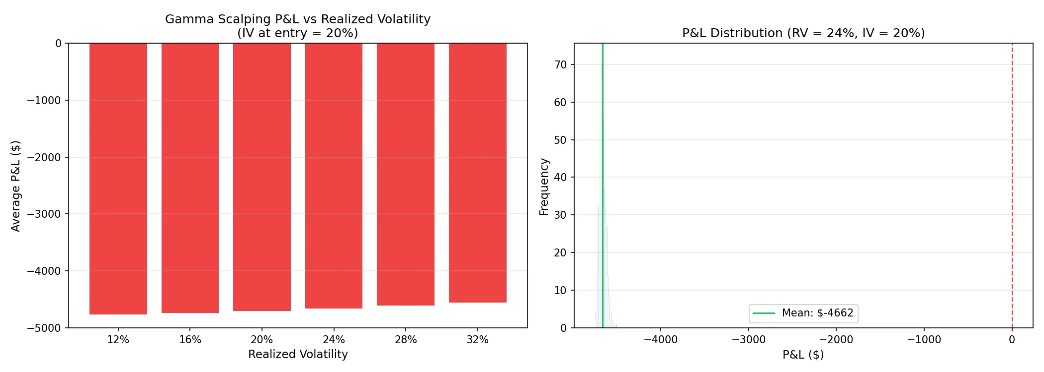
Key takeaways from the simulation:
When realized volatility is below implied volatility (RV < IV), the strategy loses on average. At RV = 12% with IV = 20%, gamma scalping is almost guaranteed to lose because the underlying does not move enough to cover Theta.
At RV ≈ IV, it is roughly breakeven. Small profits and losses depend on path, with win rates near 50%.
When RV > IV, expected value turns positive. The larger the gap, the more you earn. RV = 28% against IV = 20% is a comfortable profit zone.
When to Use Gamma Scalping
Most of the time, implied volatility exceeds realized volatility (this is why the VRP exists), making gamma scalping negative expected value on average. Blindly buying straddles and hedging will lose money over time.
Windows where gamma scalping has positive expectation:
Before earnings. If a stock’s straddle-implied move is pricing less than the historical average earnings move, buying the straddle and scalping gamma has an edge.
Before macro events. If the VIX term structure is steep with short-term implied vol unusually low relative to history, the market may be underpricing near-term movement.
Volatility mean reversion from extremes. When IV Percentile is at rock bottom (< 10%), historically IV tends to snap back. Buying options captures both Gamma profits and Vega gains from IV expansion.
Avoid opening gamma scalps when IV Rank is already elevated. You are paying a high price for volatility and need even more extreme realized moves to break even.