Fama-French Factor Model: From Three Factors to Five

A stock returned 20% last year. How much of that came from the overall market rising, how much from it being a small-cap, and how much from it being cheap? The Fama-French factor model is the tool that answers this question. It decomposes stock returns into a handful of explainable “factors” and forms a foundational framework for quantitative stock selection. This article starts from CAPM, builds up to the three-factor and five-factor models, and runs a factor regression in Python.

CAPM: A One-Factor World

Before Fama-French, finance explained stock returns with the Capital Asset Pricing Model (CAPM):

In plain terms: a stock’s expected return = risk-free rate + its sensitivity to the market (β) × the market risk premium.

Stocks with β > 1 swing more than the market, bear more risk, and are compensated with higher expected returns. Stocks with β < 1 do the opposite. CAPM’s worldview is clean: differences in stock returns come from one thing only, how much market risk a stock carries.

The problem? Real data disagreed.

In 1981, Banz found that small-cap stocks earned significantly higher long-run returns than large-caps, more than their betas could justify. In 1992, Fama and French showed that stocks with high book-to-market ratios (B/M) outperformed low-B/M stocks over long horizons. These two patterns, the size premium and the value premium, were anomalies that CAPM could not explain.

One factor was not enough. So they added more.

Three-Factor Model: Size and Value

In 1993, Fama and French extended CAPM by adding two new factors:

The three factors:

MKT (Market factor), the same \(R_m - R_f\) from CAPM. If the market rises 1% and your \(\beta_1 = 1.2\), this factor contributes 1.2% to your return.

SMB (Small Minus Big, size factor). Split all stocks into two groups by market cap. SMB is the return of the small-cap portfolio minus the large-cap portfolio. A positive \(\beta_2\) means the stock behaves like a small-cap and captures the size premium.

HML (High Minus Low, value factor). Split all stocks by book-to-market ratio. HML is the return of the high-B/M (cheap) portfolio minus the low-B/M (expensive) portfolio. A positive \(\beta_3\) means the stock has value characteristics.

The \(\alpha_i\) on the left side is the key output: it represents excess return that none of the three factors can explain. If a fund manager’s α is significantly positive, it means genuine stock-picking skill. Conversely, many funds with impressive headline returns show α near zero once you strip out factor exposures. Their returns could be replicated with a combination of cheap ETFs, at least in theory.

How Factors Are Constructed

Fama and French’s original method: at the end of each June, sort all stocks by market cap median into Big and Small; simultaneously sort by B/M ratio at 30th/70th percentiles into High, Medium, and Low. That gives 2 × 3 = 6 portfolios.

• SMB = average return of the three small portfolios minus the three big portfolios
• HML = average return of the two high-B/M portfolios minus the two low-B/M portfolios

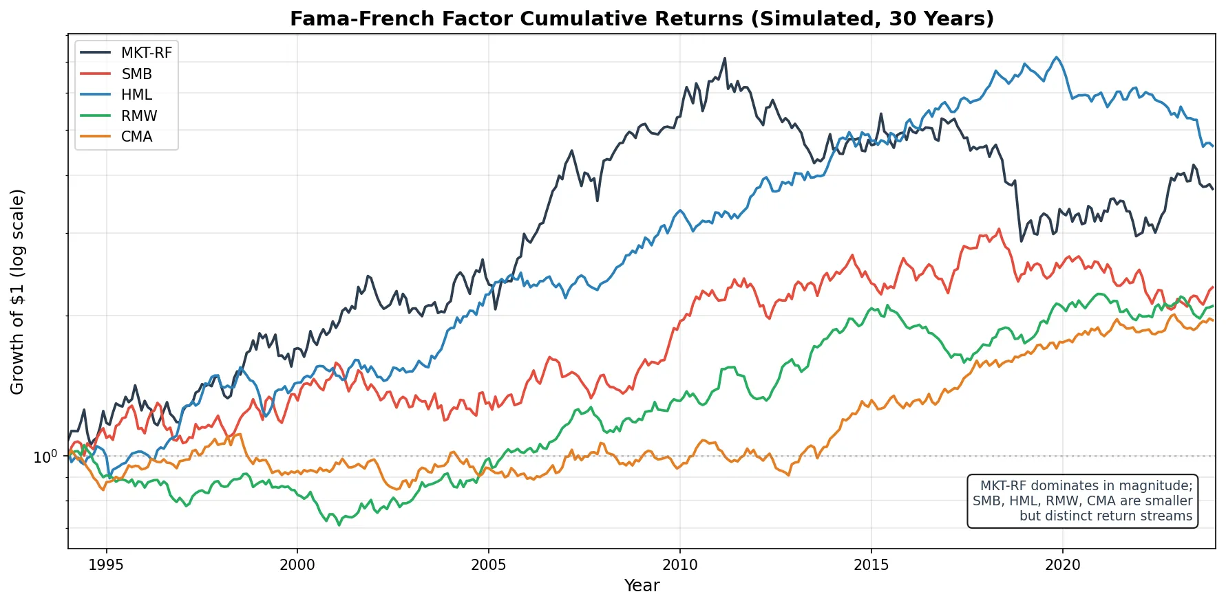
This long-short construction means factor returns represent a style premium independent of the overall market direction.

Five-Factor Model: Profitability and Investment

The three-factor model captured size and value effects, but some anomalies remained. Two companies with similar market cap and valuation can have very different long-run returns. Why? Novy-Marx showed in 2013 that gross profitability predicts stock returns. Fama and French incorporated profitability and investment patterns into a five-factor model in their 2015 paper:

The two new factors:

RMW (Robust Minus Weak, profitability factor). Return of high-profitability firms minus low-profitability firms. The intuition is straightforward: companies that earn more tend to outperform.

CMA (Conservative Minus Aggressive, investment factor). Return of firms that invest conservatively (low asset growth) minus firms that invest aggressively (high asset growth). This sounds counterintuitive, but the data shows that companies on expansion sprees tend to overinvest, depress their returns on capital, and underperform in the long run.

An interesting side effect: once RMW and CMA are included, HML’s explanatory power weakens considerably. Fama and French themselves acknowledged that HML becomes nearly redundant in the five-factor model, because much of the value effect can be explained by profitability and investment patterns. This sparked academic debate: is value investing an independent risk premium, or just a byproduct of profitability and investment style?

Python Factor Regression

Theory aside, here is a working implementation. We simulate monthly returns for a “small-cap value fund” and run both three-factor and five-factor regressions. In practice, factor data is available for free from Kenneth French’s Data Library. The code below uses synthetic data to keep it self-contained.

import numpy as np
from numpy.linalg import lstsq

def run_factor_regression():
    np.random.seed(42)
    n = 240  # 20 years of monthly data

    # Simulate factor returns (monthly)
    mkt = np.random.normal(0.007, 0.045, n)
    smb = np.random.normal(0.002, 0.032, n)
    hml = np.random.normal(0.003, 0.028, n)
    rmw = np.random.normal(0.0025, 0.022, n)
    cma = np.random.normal(0.002, 0.020, n)

    # Simulate fund returns: small-cap value fund
    # True betas: MKT=1.05, SMB=0.45, HML=0.38, RMW=0.18, CMA=0.12
    # True alpha: 0.001 (0.1% per month)
    alpha_true = 0.001
    fund = (alpha_true + 1.05 * mkt + 0.45 * smb + 0.38 * hml
            + 0.18 * rmw + 0.12 * cma + np.random.normal(0, 0.012, n))

    # --- Three-factor regression ---
    X3 = np.column_stack([np.ones(n), mkt, smb, hml])
    beta3, residuals3, _, _ = lstsq(X3, fund, rcond=None)
    pred3 = X3 @ beta3
    ss_res3 = np.sum((fund - pred3) ** 2)
    ss_tot = np.sum((fund - np.mean(fund)) ** 2)
    r2_3 = 1 - ss_res3 / ss_tot

    # Standard errors
    mse3 = ss_res3 / (n - 4)
    se3 = np.sqrt(np.diag(mse3 * np.linalg.inv(X3.T @ X3)))
    t3 = beta3 / se3

    print("=== Three-Factor Model ===")
    print(f"  Alpha:  {beta3[0]*100:.3f}% /month  (t={t3[0]:.2f})")
    print(f"  MKT:    {beta3[1]:.3f}  (t={t3[1]:.2f})")
    print(f"  SMB:    {beta3[2]:.3f}  (t={t3[2]:.2f})")
    print(f"  HML:    {beta3[3]:.3f}  (t={t3[3]:.2f})")
    print(f"  R²:     {r2_3:.4f}")

    # --- Five-factor regression ---
    X5 = np.column_stack([np.ones(n), mkt, smb, hml, rmw, cma])
    beta5, _, _, _ = lstsq(X5, fund, rcond=None)
    pred5 = X5 @ beta5
    ss_res5 = np.sum((fund - pred5) ** 2)
    r2_5 = 1 - ss_res5 / ss_tot

    mse5 = ss_res5 / (n - 6)
    se5 = np.sqrt(np.diag(mse5 * np.linalg.inv(X5.T @ X5)))
    t5 = beta5 / se5

    print("\n=== Five-Factor Model ===")
    print(f"  Alpha:  {beta5[0]*100:.3f}% /month  (t={t5[0]:.2f})")
    print(f"  MKT:    {beta5[1]:.3f}  (t={t5[1]:.2f})")
    print(f"  SMB:    {beta5[2]:.3f}  (t={t5[2]:.2f})")
    print(f"  HML:    {beta5[3]:.3f}  (t={t5[3]:.2f})")
    print(f"  RMW:    {beta5[4]:.3f}  (t={t5[4]:.2f})")
    print(f"  CMA:    {beta5[5]:.3f}  (t={t5[5]:.2f})")
    print(f"  R²:     {r2_5:.4f}")
    print(f"\n  R² improvement: {r2_3:.4f} -> {r2_5:.4f} (+{(r2_5-r2_3)*100:.2f}%)")

run_factor_regression()

Output:

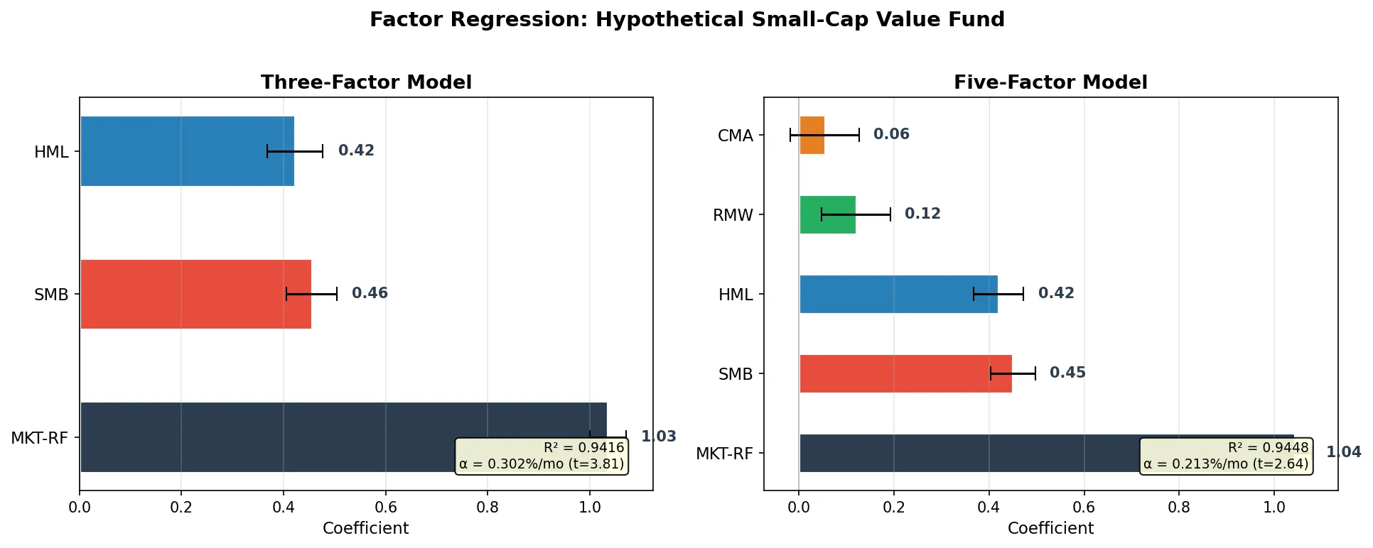
=== Three-Factor Model ===
  Alpha:  0.302% /month  (t=3.81)
  MKT:    1.035  (t=57.98)
  SMB:    0.455  (t=18.49)
  HML:    0.422  (t=15.20)
  R²:     0.9416

=== Five-Factor Model ===
  Alpha:  0.213% /month  (t=2.64)
  MKT:    1.043  (t=59.28)
  SMB:    0.450  (t=18.67)
  HML:    0.420  (t=15.47)
  RMW:    0.121  (t=3.27)
  CMA:    0.055  (t=1.49)
  R²:     0.9448

  R² improvement: 0.9416 -> 0.9448 (+0.32%)

Key observations:

MKT coefficient of 1.04, close to the true value of 1.05. t-stat near 60, highly significant. This “fund” basically tracks the market.

SMB coefficient of 0.45, significantly positive, confirming the small-cap tilt. If you bought a fund marketed as “large-cap blue chip” and the regression shows SMB significantly positive, the manager is actually buying small-caps. Factor regression catches style drift.

Three-factor α is 0.302%/month with t = 3.81, statistically significant. Under the five-factor model, α drops to 0.213% with t = 2.64. Part of the “unexplained” excess return was actually RMW and CMA factor exposure. This is the core use of factor models: peel away factor exposures, then see how much genuine α remains.

R² goes from 0.9416 to 0.9448. The five-factor model explains an additional 0.32% of return variance. Not much, but RMW’s t-stat of 3.27 is significant, meaning the profitability factor has independent explanatory power. CMA’s t-stat of 1.49 is not significant in this sample.

Limitations of Factor Models

Factor models have blind spots.

Factor premiums can disappear. The small-cap premium was a cornerstone of the three-factor model, but it has weakened substantially in US equities since the 1980s, and has been negative in some periods. One explanation: once academic papers publicized the anomaly, capital flooded into small-cap strategies and arbitraged the premium away. Factor crowding is a long-term threat to any factor strategy.

Factors do not port across markets automatically. Fama-French factors were discovered on US data. In China’s A-share market, the size effect (small-caps outperforming) remains strong, but the value effect (cheap stocks outperforming) has been persistently weak. Many “cheap” A-share stocks are fundamentally deteriorating. Applying US-derived factor models directly to other markets without local validation is risky.

Data mining is rampant. Academics have “discovered” hundreds of factors (one count puts the number above 400). Many are significant only in specific time periods or markets and vanish out of sample. Harvey, Liu & Zhu (2016) showed that the traditional t > 2 threshold produces a flood of false positives under multiple testing.

Linearity assumption. Factor models assume a linear relationship between returns and factors. In reality, the size premium might concentrate in the bottom decile of stocks rather than increasing linearly as size decreases.

Factor Models and Quant Stock Selection

Factor models are not just analytical tools. They are the theoretical foundation for quantitative stock selection.

The most direct application is factor-based stock picking. If you believe the value factor works, systematically buy high-B/M stocks and sell low-B/M stocks. If you believe in multiple factors, combine them into a multi-factor scoring model. Chinese quant hedge funds’ “multi-factor models” are built on exactly this logic.

Factor attribution is another use. A fund manager claims 25% annual returns. Factor regression might reveal: 18% from the market, 4% from small-cap exposure, 2% from value exposure, and only 1% in genuine α. Would you pay a 2% management fee for 1% of α? This is what factor attribution answers.

Factor neutrality takes it further. Some strategies want zero factor risk, pure α. The method: when constructing a portfolio, constrain exposure to each factor to zero. Go long a set of stocks while shorting an equal amount with opposite factor exposures, making the portfolio’s SMB, HML, and other coefficients close to zero. What remains is pure stock-picking ability, uncorrelated with any known factor.

The math behind factor models is just multivariate linear regression. The hard parts are choosing which factors to use, handling correlations between factors, dynamically adjusting factor weights, and avoiding overfitting to historical data.