Dispersion trading is one of the few options strategies with a persistent structural edge. The core trade is straightforward: sell index options, buy component stock options. You are not betting on direction or volatility level. You are betting that index implied correlation overstates the actual co-movement of constituent stocks.
This edge exists because institutional investors have a structural, ongoing need for portfolio downside protection. They buy index puts, which inflates index implied volatility and, by extension, implied correlation. Dispersion traders earn a premium by bearing the tail risk of correlation spiking to 1.0 during a crisis.
The Core Logic of Dispersion Trading
Pairs trading bets on spread reversion between two stocks. Dispersion trading bets on the “scatter” among a basket of stocks diverging from what index option prices imply. In pairs trading, you bet two stocks will revert to their normal relationship. In dispersion trading, you bet that component stocks will not move in lockstep.
The execution: sell an ATM straddle on the S&P 500 index (SPX), and simultaneously buy ATM straddles on 15–30 of the largest index components. The index leg collects premium; the component legs spend premium. If constituents move independently (low correlation), the gains from individual stock straddles cover the index leg’s losses. If all stocks crash together (high correlation), the index leg blows up.
Put simply, dispersion trading is a short correlation bet.
Why “dispersion”? When component stocks diverge (high dispersion), the index itself barely moves: A is up 3%, B is down 2%, C is flat, so the index moves 0.5%. Your short index straddle loses little, and at least a few of your long stock straddles pay off. When stocks move in unison, dispersion is low, correlation is high, and the index leg suffers.
Variance Decomposition: The Math Behind Dispersion Trading
Dispersion trading has a solid mathematical foundation. An index’s variance decomposes into two components: the individual stock variances, plus the cross-covariance terms.
For an index with \(n\) components, where stock \(i\) has weight \(w_i\), volatility \(\sigma_i\), and the correlation between stocks \(i\) and \(j\) is \(\rho_{ij}\):
$$\sigma_{\text{index}}^2 = \sum_{i=1}^{n} w_i^2 \sigma_i^2 + \sum_{i \neq j} w_i w_j \rho_{ij} \sigma_i \sigma_j$$The first term captures each stock’s standalone variance contribution. The second term captures the co-movement contribution. When stocks are uncorrelated (\(\rho_{ij} = 0\)), the second term vanishes and index variance is far smaller than the weighted sum of component variances.
This explains a well-known fact in options markets: index implied volatility is always lower than the weighted average of component implied volatilities. Diversification compresses index-level volatility.
Computing Implied Correlation
Assuming a uniform pairwise correlation \(\bar{\rho}\) across all components, the variance formula simplifies to:
$$\sigma_{\text{index}}^2 = \bar{\rho} \left(\sum_i w_i \sigma_i\right)^2 + (1 - \bar{\rho}) \sum_i w_i^2 \sigma_i^2$$Solving for \(\bar{\rho}\):
$$\bar{\rho}_{\text{implied}} = \frac{\sigma_{\text{index}}^2 - \sum_i w_i^2 \sigma_i^2}{\left(\sum_i w_i \sigma_i\right)^2 - \sum_i w_i^2 \sigma_i^2}$$Plug in index implied volatility for \(\sigma_{\text{index}}\) and component implied volatilities for \(\sigma_i\), and you get the market-implied correlation level.
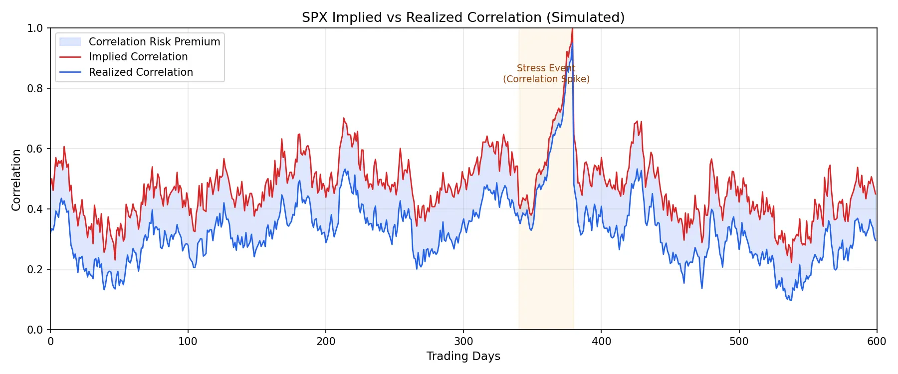
The key observation: on the S&P 500, implied correlation persistently exceeds realized correlation by roughly 10–20 percentage points. In normal markets, implied correlation runs 40%–60% while realized correlation hovers at 25%–40%. This gap is the dispersion trader’s profit source.
Why Implied Correlation Is Persistently Elevated
This is not a market mispricing. Institutional investors need portfolio protection, and the most capital-efficient hedge is buying SPX puts rather than hedging each stock individually. This concentrated demand pushes index implied volatility higher, which mathematically inflates implied correlation.
The implied correlation premium is a risk premium. Dispersion traders earn it by absorbing the tail risk of “all stocks crashing together.” Similar to the volatility risk premium that short-vol traders harvest, dispersion traders capture the correlation risk premium (CRP).
Portfolio Construction: Building a Dispersion Trade
The Index Leg
The most common choice is selling SPX ATM straddles with 30-day expiry. Alternatives include strangles (which reduce Gamma exposure) or variance swaps (which isolate pure variance exposure without strike selection bias). Variance swaps are the cleanest instrument but are only accessible in the institutional OTC market.
For retail execution, selling monthly SPX straddles is the most direct route.
The Component Leg
You do not need to buy options on all 500 index components. Select the 15–30 largest by weight, covering 40%–60% of the index. Selection criteria: large weight and good options liquidity. The usual suspects are AAPL, MSFT, AMZN, NVDA, GOOGL, and META.
Buy ATM straddles on each component, matching the index leg’s expiry.
Vega Weighting
This step separates a proper dispersion trade from a naive “sell index, buy stocks” position. The portfolio must be Vega-neutral at inception: you are not making a directional volatility bet, only a correlation bet.
Vega measures an option’s price sensitivity to a 1-percentage-point change in implied volatility. Vega neutrality means: if all implied volatilities shift up or down by the same amount, the portfolio P&L is zero.
The calculation: compute the total Vega exposure of the short index position (e.g., -$50,000/vol point), then allocate this Vega across components by weight. The number of straddles to buy for component \(i\):
$$N_i = \frac{w_i \times |\text{Vega}_{\text{index}}|}{\text{Vega}_i^{\text{per straddle}}}$$where \(w_i\) is the component’s index weight and \(\text{Vega}_i^{\text{per straddle}}\) is the Vega of one straddle on that stock.
Delta Hedging
After establishing the position, hedge the index leg’s Delta with SPX futures and each component’s Delta with its own stock. Hedging frequency depends on your Gamma risk tolerance. Institutional desks typically hedge daily; some run continuous intraday hedges. Retail traders using monthly options can rebalance Delta every few days.
A Concrete Example
Suppose SPX 30-day ATM straddle implied volatility is 18%, and the weighted average 30-day implied volatility of the top 20 components is 25%. Plugging into the implied correlation formula yields implied correlation of roughly 0.52.
Over the same period, the 30-day realized correlation of these 20 stocks is 0.35.
Gap = 0.52 - 0.35 = 0.17. This is your potential profit margin. As long as realized correlation stays below 0.52 during the holding period, the trade is profitable.
Dispersion Trading vs Correlation Trading
Dispersion trading is often conflated with “correlation trading,” but the two differ in execution.
| Dimension | Dispersion Trading | Correlation Trading |
|---|---|---|
| Instruments | Index options + stock options | Correlation swaps |
| Exposure | Correlation + partial vol exposure | Pure correlation |
| Execution complexity | High (multi-leg management) | Low (single trade) |
| Liquidity | Good (listed options) | Poor (OTC derivatives) |
| Suitable for | Institutional desks, advanced retail | Institutional only |
| Nonlinearity | Yes (straddles carry Gamma) | Linear payoff |
Dispersion trading does not perfectly isolate correlation exposure. Because you replicate variance positions with options, the options carry Gamma, Theta, and other Greeks. Variance swaps provide cleaner isolation but are inaccessible to retail. In practice, dispersion trading profits come partly from the correlation premium and partly from the volatility risk premium.
Risk Management: How Dispersion Trades Fail
Correlation Spikes
During the 2008 financial crisis and the March 2020 COVID crash, SPX component realized correlations surged above 0.8. All stocks fell together, and component straddle gains were nowhere near enough to cover index leg losses. Quantpedia’s backtest data shows maximum drawdowns exceeding 40% for dispersion strategies in 2008.
This is the fundamental risk: you earn steady premiums in normal times and suffer tail losses in crises. Like selling insurance: you profit 95% of the time, but one event can wipe out years of gains.
Liquidity Risk
Individual stock option bid-ask spreads are much wider than index option spreads. Managing 20 straddle positions across different names, the slippage alone can erode a significant portion of profits. Smaller-cap components have even worse liquidity, which is why practitioners limit the basket to the top 15–30 names.
Gamma and Pin Risk
Near expiration, Gamma exposure increases sharply. If a component stock hovers around its strike (pin risk), Delta hedging becomes extremely difficult. Institutional desks typically start closing or rolling positions one week before expiry to avoid the last few days of Gamma risk.
Transaction Costs
Twenty component straddles plus one index straddle plus ongoing Delta hedging. Every rebalance incurs commissions and slippage. Gross returns on this strategy typically run 8%–15% annualized; poor cost management can halve the net return.
Python: Computing Implied Correlation Signals
The code below computes rolling realized correlation for SPX components and generates a Z-score signal. This is not a full backtest (real dispersion trading requires options price data unavailable from free sources) but a signal framework for gauging whether conditions favor dispersion trades.
import numpy as np
import pandas as pd
import yfinance as yf
import matplotlib.pyplot as plt

# --- 1. Download top SPX components ---
top20 = [
    "AAPL", "MSFT", "NVDA", "AMZN", "GOOGL",
    "META", "BRK-B", "AVGO", "LLY", "JPM",
    "TSLA", "UNH", "V", "XOM", "MA",
    "COST", "PG", "JNJ", "HD", "ABBV"
]

data = yf.download(top20, start="2024-01-01", end="2026-06-30")["Close"]

# --- 2. Compute rolling realized correlation ---
returns = np.log(data / data.shift(1)).dropna()

def rolling_avg_correlation(returns_df, window=30):
    """Compute the average pairwise correlation over a rolling window."""
    result = []
    for i in range(window, len(returns_df)):
        window_ret = returns_df.iloc[i-window:i]
        corr_matrix = window_ret.corr()
        n = len(corr_matrix)
        mask = np.triu(np.ones((n, n), dtype=bool), k=1)
        avg_corr = corr_matrix.values[mask].mean()
        result.append({
            "date": returns_df.index[i],
            "avg_correlation": avg_corr
        })
    return pd.DataFrame(result).set_index("date")

realized_corr = rolling_avg_correlation(returns, window=30)

# --- 3. Visualize ---
fig, ax = plt.subplots(figsize=(12, 5))
ax.plot(realized_corr.index, realized_corr["avg_correlation"],
        color="#2563eb", linewidth=1.2, label="30-Day Realized Correlation (Top 20)")
ax.axhline(y=realized_corr["avg_correlation"].mean(), color="#9ca3af",
           linestyle="--", linewidth=0.8, label="Mean")
ax.set_ylabel("Average Pairwise Correlation")
ax.set_title("SPX Top-20 Components: 30-Day Rolling Realized Correlation")
ax.legend(loc="upper right")
ax.set_ylim(0, 1)
ax.grid(True, alpha=0.3)
plt.tight_layout()
plt.savefig("realized-correlation-rolling.webp", dpi=150)
plt.show()

# --- 4. Signal logic ---
mean_corr = realized_corr["avg_correlation"].mean()
std_corr = realized_corr["avg_correlation"].std()

realized_corr["z_score"] = (
    (realized_corr["avg_correlation"] - mean_corr) / std_corr
)

realized_corr["signal"] = np.where(
    realized_corr["z_score"] < -1, "favorable",
    np.where(realized_corr["z_score"] > 1, "dangerous", "neutral")
)

print("\nDispersion trading signal distribution:")
print(realized_corr["signal"].value_counts(normalize=True).round(3))
print(f"\nMean realized correlation: {mean_corr:.3f}")
print(f"Current realized correlation: "
      f"{realized_corr['avg_correlation'].iloc[-1]:.3f}")
print(f"Current Z-score: {realized_corr['z_score'].iloc[-1]:.2f}")
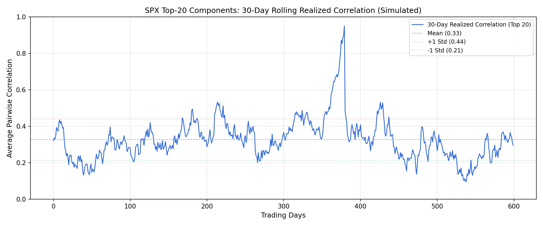
The code does three things: fetches data, computes 30-day rolling average pairwise correlation, and generates a Z-score signal. When the Z-score drops below -1 (realized correlation well below average), conditions favor dispersion trades because stocks are moving independently. When it exceeds +1, correlation is elevated and tail risk is heightened.
In live trading, you would also compute implied correlation from the options chain and compare it against realized correlation. The wider the gap, the stronger the signal. The CBOE publishes implied correlation indices (ICJ, JCJ) as a rough proxy, but professional desks compute their own from real-time option prices.
Can Retail Traders Do Dispersion Trading?
Honestly, full-scale dispersion trading is not well-suited for retail accounts. Twenty component straddles plus one index straddle require six-figure USD margin. Add daily Delta hedging and monthly rolls, and the operational complexity and transaction costs stack up.
But the core signal, the gap between implied and realized correlation, is useful for any options trader. A few simplified approaches:
Scale down. Instead of 20 stocks, pick the 5 largest components and use SPY instead of SPX. Smaller positions, same core logic, lower precision but much lower costs.
Signal only. Do not execute a dispersion trade directly, but use the correlation signal to time short-volatility strategies. When realized correlation is low, selling SPX volatility is safer because stocks are unlikely to crash simultaneously.
Use sector ETFs. Replace individual stocks with sector ETFs like XLK (tech) or XLF (financials). Fewer legs, much lower transaction costs, though less precise than single-stock straddles.
When to stay away: VIX above 30, or when implied correlation is already elevated. In risk-off environments, correlation can spike further, and shorting correlation is like selling umbrellas in a hurricane.