CTA (Commodity Trading Advisor) is a broad category of quantitative strategies that trade futures. Despite the name suggesting commodities only, CTA strategies cover equity index futures, treasury futures, and FX futures as well. The space splits into two camps: trend following (go long when prices rise, short when they fall) and statistical arbitrage (find mispricings between related instruments and bet on convergence). This article covers both, with Python code for each.
Three Types of CTA Strategies
CTA strategies fall into three buckets based on trading logic.
Trend following dominates the CTA world. Over 70% of managed futures assets globally run some form of trend following. The logic is simple: if a market is going up, go long; if it is going down, go short. The philosophy is “cut losses short, let profits run.” The core assumption behind trend following is that price momentum persists: markets that have been rising are more likely to continue rising in the near term than to reverse.
Statistical arbitrage / mean reversion takes the opposite approach: find two correlated instruments whose price spread has deviated from its historical norm, short the expensive one, buy the cheap one, and wait for the spread to normalize. This strategy does not bet on market direction. It bets on relationships reverting to normal.
High-frequency market making earns the bid-ask spread by providing liquidity. It requires extreme low-latency infrastructure and is outside the scope of this article.
Trend following and statistical arbitrage are nearly opposite mindsets, suited to different market environments:
| Trend Following | Statistical Arbitrage | |
|---|---|---|
| Core logic | Momentum persists | Deviations revert |
| Win rate | Low (30-40%) | High (60-70%) |
| Profit/loss ratio | High (big wins) | Low (limited per trade) |
| Best market | Strong trends | Range-bound, choppy |
| Drawdown source | Whipsaws in choppy markets | Spread divergence (broken relationships) |
| Typical Sharpe | 0.3 - 0.8 | 1.0 - 2.0 |
CTA strategies have a property that institutional investors value: crisis alpha. During the 2008 financial crisis, global equity markets crashed, but trend following strategies profited by shorting equity index and commodity futures. The SG Trend Index returned +21% in 2008 while the S&P 500 fell 37%. This negative correlation with equities makes CTA a “portfolio insurance” allocation for institutions.
Trend Following: Dual Moving Average Crossover
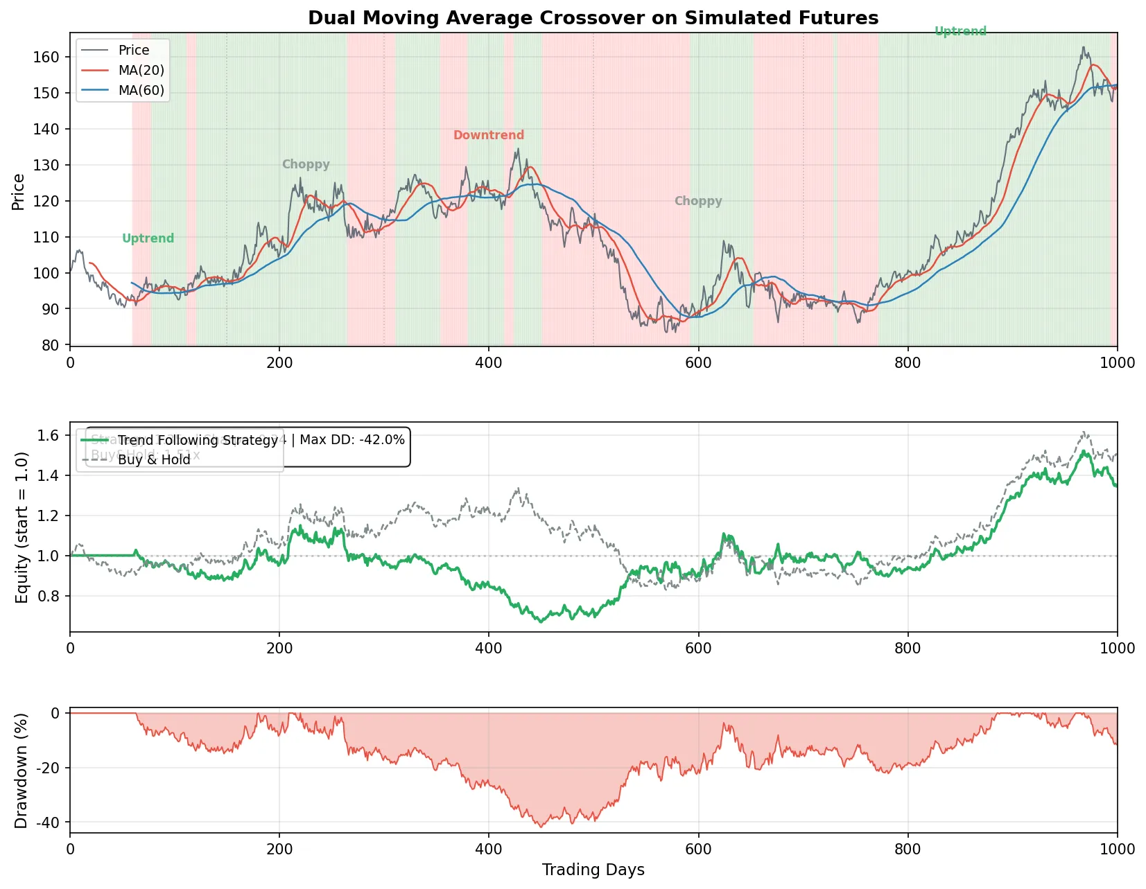
The most classic trend following implementation is the moving average crossover. Use two moving averages with different lookback periods: one short (e.g., 20 days), one long (e.g., 60 days). When the short MA crosses above the long MA (“golden cross”), recent momentum is up, go long. When the short MA crosses below (“death cross”), go short.
Parameter intuition: the short MA filters out daily noise and captures recent trend direction. The long MA confirms the broader trend. If the short MA is too short (e.g., 5 days), every random fluctuation triggers a signal and you get whipsawed constantly. If the long MA is too long (e.g., 200 days), signals come too late and the trend is already over by the time you enter. The 20/60 combination is a common medium-frequency choice.
The following Python code simulates a futures price series with alternating trend and choppy regimes, then runs a dual MA crossover strategy:
import numpy as np

def simulate_trend_following(n_days=1000, short_window=20, long_window=60):
    np.random.seed(42)

    # Simulated futures price: 5 phases alternating trend and choppy
    regimes = [
        (0, 150, 0.0008, 0.012),     # uptrend
        (150, 300, -0.0001, 0.018),   # choppy
        (300, 500, -0.0006, 0.013),   # downtrend
        (500, 700, 0.0001, 0.020),    # choppy
        (700, 1000, 0.0007, 0.011),   # uptrend
    ]

    returns = np.zeros(n_days)
    for start, end, mu, sigma in regimes:
        returns[start:end] = np.random.normal(mu, sigma, end - start)

    price = 100 * np.exp(np.cumsum(returns))

    # Compute moving averages
    ma_short = np.array([np.mean(price[max(0, i-short_window+1):i+1])
                         if i >= short_window - 1 else np.nan
                         for i in range(n_days)])
    ma_long = np.array([np.mean(price[max(0, i-long_window+1):i+1])
                        if i >= long_window - 1 else np.nan
                        for i in range(n_days)])

    # Signal: long when short MA > long MA, short otherwise
    position = np.zeros(n_days)
    for i in range(long_window, n_days):
        position[i] = 1 if ma_short[i] > ma_long[i] else -1

    # Strategy returns
    strategy_ret = position[:-1] * returns[1:]
    strategy_ret = np.insert(strategy_ret, 0, 0)
    strategy_equity = np.exp(np.cumsum(strategy_ret))
    buyhold_equity = price / price[0]

    # Stats
    active_ret = strategy_ret[long_window:]
    sharpe = np.mean(active_ret) / np.std(active_ret) * np.sqrt(252)
    peak = np.maximum.accumulate(strategy_equity)
    max_dd = np.min((strategy_equity - peak) / peak)

    print(f"Strategy final equity: {strategy_equity[-1]:.2f}x")
    print(f"Buy & Hold final equity: {buyhold_equity[-1]:.2f}x")
    print(f"Sharpe ratio: {sharpe:.2f}")
    print(f"Max drawdown: {max_dd:.1%}")

simulate_trend_following()
Results:
Strategy final equity: 1.35x
Buy & Hold final equity: 1.51x
Sharpe ratio: 0.34
Max drawdown: -42.0%
| Final Equity | Sharpe | Max Drawdown | Win Rate | Avg W/L Ratio | |
|---|---|---|---|---|---|
| Trend Following | 1.35x | 0.34 | -42.0% | 35.3% | 2.6:1 |
| Buy & Hold | 1.51x | - | - | - | - |
The simulation triggered 17 trades total, only 6 of which were profitable, for a 35.3% win rate. But winning trades averaged 2.6 times the size of losing trades. This is the signature pattern of trend following: most of the time you are losing small amounts (choppy markets trigger repeated crossovers and stops), while a few large trends generate profits that cover all the losses.
The Achilles Heel of Trend Following
The simulation shows strategy equity (1.35x) actually trails buy and hold (1.51x). That is not because trend following is broken. It is because choppy periods account for nearly half the simulation. Choppy markets are trend following’s worst enemy: no clear direction, MAs cross back and forth repeatedly, and the strategy keeps entering and exiting at a loss. This cumulative drag is called the “trend tax.”
The profit distribution is extremely concentrated: out of 17 trades, only 6 were profitable, while the remaining 11 lost money. Miss those few big trends (say, by using different parameters that enter too late) and the total return flips negative.
Parameter sensitivity is another concern. Changing the short MA from 20 to 15 or 25 days can shift results substantially. But optimizing parameters to make the backtest look best is exactly the kind of overfitting described in the backtesting pitfalls guide. The practical approach: use the same parameter set across many instruments and rely on diversification across instruments to smooth out single-instrument parameter risk.
ATR Position Sizing
Trend following strategies typically pair with ATR (Average True Range) for position sizing. ATR measures the average daily price range over the last N days. Volatile instruments (e.g., crude oil, with daily swings of 3%) get smaller positions; low-volatility instruments (e.g., treasury futures, with 0.3% daily swings) get larger positions.
A common rule: risk per trade = 1 ATR equals 1% of total capital. If the account has $1 million and 1% is $10,000, and an instrument’s ATR is 50 ticks at $10 per tick, the maximum position is $10,000 / (50 x $10) = 20 contracts. This normalizes risk across all instruments regardless of their volatility.
TA-Lib’s ATR function computes this indicator directly.
Futures Spread Arbitrage
CTA arbitrage strategies use the same methodology as pairs trading: test for cointegration, construct a spread, enter when the spread deviates, exit when it reverts. The difference is that the instruments are futures contracts, and the arbitrage types fall into two main categories.
Calendar Spread Arbitrage
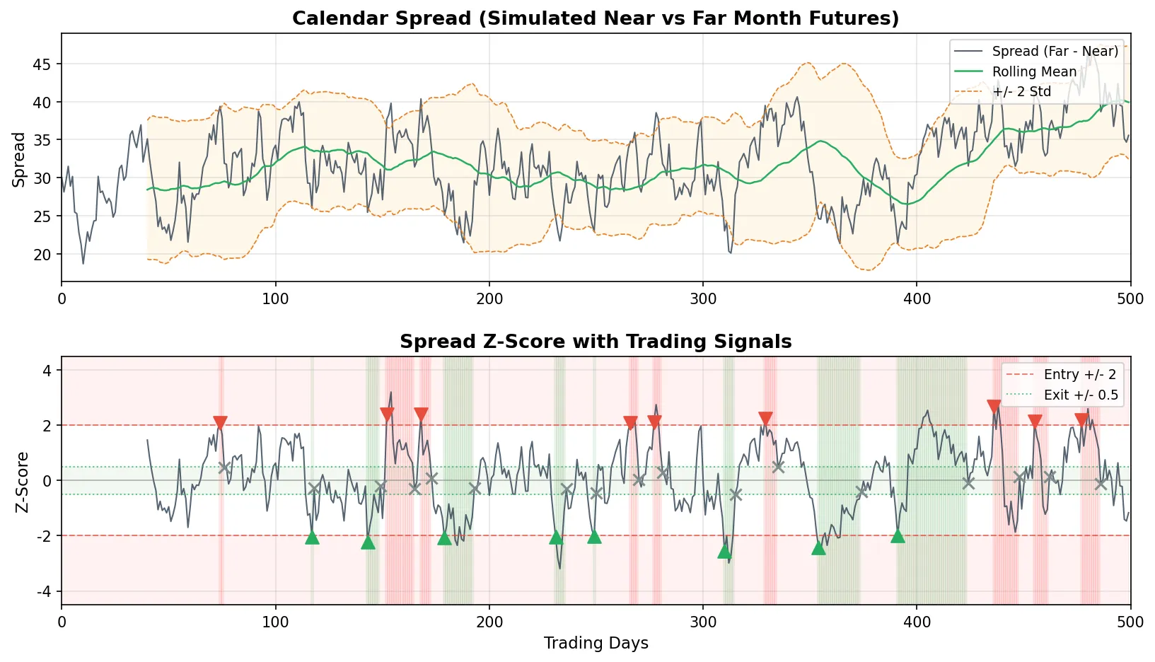
Calendar spread (or time spread) trades the price difference between two contracts of the same commodity with different expiration months. For example, crude oil May 2025 vs. October 2025. Both track the same underlying, but their price difference reflects carrying costs (storage, interest rates) and market expectations about future supply and demand.
Under normal conditions, the far-month contract trades at a premium to the near-month (contango), and the spread is relatively stable. When the spread deviates due to short-term supply shocks, approaching delivery dates, or shifts in the term structure, arbitrage opportunities arise.
Intercommodity Spread Arbitrage
Intercommodity spread trades the price difference between two different but related commodities. Classic examples:
- Soybean crush spread: soybean meal + soybean oil vs. soybeans. The physical crushing process links the three, and spread deviations signal abnormal processing margins
- Steel vs. iron ore: upstream-downstream relationship in steel production, spread represents mill profitability
- WTI vs. Brent crude: two regional crude benchmarks, spread driven by regional supply/demand and shipping costs
Signal Generation: Z-Score Method
Whether calendar or intercommodity, the signal logic is the same: compute a rolling Z-score of the spread and enter when it exceeds a threshold.
import numpy as np

def simulate_calendar_spread():
    np.random.seed(123)
    n = 500

    # Simulate two correlated futures contracts (near vs far month)
    common = np.cumsum(np.random.normal(0.0002, 0.012, n))
    near = 3500 + common * 100 + np.cumsum(np.random.normal(0, 0.8, n))

    # Far month = near + contango premium + mean-reverting noise
    spread_noise = np.zeros(n)
    for i in range(1, n):
        spread_noise[i] = 0.93 * spread_noise[i-1] + np.random.normal(0, 2.5)
    far = near + 30 + spread_noise

    spread = far - near
    lookback = 40

    # Rolling Z-score
    z_score = np.full(n, np.nan)
    for i in range(lookback, n):
        window = spread[i-lookback:i]
        std_w = np.std(window)
        if std_w > 0:
            z_score[i] = (spread[i] - np.mean(window)) / std_w

    # Signals
    position = np.zeros(n)
    for i in range(lookback + 1, n):
        if np.isnan(z_score[i]):
            position[i] = position[i-1]
            continue
        if position[i-1] == 0:
            if z_score[i] > 2:    position[i] = -1   # spread too wide, short it
            elif z_score[i] < -2: position[i] = +1   # spread too narrow, long it
        elif position[i-1] == 1:
            if abs(z_score[i]) < 0.5:  position[i] = 0    # reverted, close
            elif z_score[i] < -4:      position[i] = 0    # stop loss
            else:                      position[i] = 1
        elif position[i-1] == -1:
            if abs(z_score[i]) < 0.5:  position[i] = 0
            elif z_score[i] > 4:       position[i] = 0
            else:                      position[i] = -1

    # P&L
    spread_ret = np.diff(spread)
    start = lookback + 1
    daily_pnl = position[start:-1] * spread_ret[start:]
    daily_pnl = daily_pnl[~np.isnan(daily_pnl)]
    n_trades = int(np.sum(np.abs(np.diff(position[start:])) > 0))

    print(f"Cumulative P&L: {np.sum(daily_pnl):.2f}")
    print(f"Trades: {n_trades} ({n_trades//2} round trips)")
    print(f"Annualized Sharpe: {np.mean(daily_pnl)/np.std(daily_pnl)*np.sqrt(252):.2f}")

simulate_calendar_spread()
Results:
Cumulative P&L: 96.14
Trades: 34 (17 round trips)
Annualized Sharpe: 2.49
17 round-trip trades, annualized Sharpe of 2.49. The cumulative P&L of 96 is in raw spread points (the spread fluctuates around a mean of roughly 32 points with a standard deviation of about 5). Compare that with trend following’s Sharpe of 0.34: arbitrage strategies have higher win rates and Sharpe ratios, but profit per trade is limited (the spread has a natural ceiling on how far it can move). Trend following, on the other hand, can generate enormous single-trade profits during large moves.
This backtest is heavily simplified: the synthetic spread is constructed to be mean-reverting by design (an AR(1) process), so we skip the cointegration test. In live trading, you must test for cointegration first, otherwise the spread may not revert at all. The code also excludes transaction costs, slippage, margin modeling, and contract rolls. Real performance would be lower. For common backtesting mistakes, see the backtesting pitfalls guide. The full Z-score implementation with cointegration testing and rolling hedge ratios is covered in the pairs trading guide.
Practical Considerations for CTA Strategies
Contract rolling. Futures contracts expire. If your trend strategy signals long on May crude oil, you need to roll the position to the October contract before May delivery. The spread between near and far month at roll time creates a cost (or occasional gain). Over years of trading, roll costs accumulate into a non-trivial drag on returns.
Margin and leverage. Futures are inherently leveraged: a 10% margin requirement means you control 10x your posted margin in notional value. If the futures price moves 1%, your margin fluctuates by 10%. CTA funds typically deploy only 20-30% of total capital as margin, parking the remaining 70-80% in treasury bills or other risk-free assets. The actual portfolio leverage is 2-3x, not the notional 10x.
Multi-instrument diversification. Any single instrument might spend months without a trend, bleeding the strategy with whipsaw losses. But if you trade 30 instruments simultaneously (equity indices, treasuries, gold, crude oil, agricultural products, metals), the probability that some subset is trending at any given time is much higher. Diversification across instruments is the primary mechanism CTA funds use to control drawdowns.
For evaluating CTA performance, the Calmar ratio (annualized return divided by the absolute value of maximum drawdown, e.g., 15% return / 30% max drawdown = 0.5) is particularly useful alongside the Sharpe ratio, because drawdown characteristics matter more in CTA than in equity strategies.
One key distinction between CTA and volatility trading strategies: volatility trading bets on whether the magnitude of price moves will exceed or fall short of market expectations. CTA bets on whether price direction will persist. The two can complement each other: CTA for directional returns, volatility strategies for risk management.