In 2016, Zura Kakushadze from WorldQuant published a six-page paper titled “101 Formulaic Alphas.” The paper did something unusual: it listed the exact formulas for 101 quantitative factors, 80 of which were running in WorldQuant’s production environment. These factors have holding periods of 0.6 to 6.4 days and an average pairwise correlation of just 15.9%.
The paper gives formulas but zero explanation. Why does Alpha#3 look the way it does? What market phenomenon is it trying to capture? Not a word. That gap is what this series fills: we classify all 101 Alpha 101 factors by their economic logic, break down the formulas, and figure out what each factor is actually betting on.
This series has five parts:
- This article: the big picture. Classification framework, operator reference, and the complete factor lookup table
- Price-volume divergence factors (32 factors)
- Momentum and reversal factors (23 factors)
- Volatility and intraday structure factors (23 factors)
- Liquidity, composite factors, and multi-factor portfolio construction (23 factors)
Data Inputs for Alpha 101
All 101 formulas draw from the same set of daily equity fields:
| Field | Meaning | Notes |
|---|---|---|
open | Opening price | |
close | Closing price | |
high | Daily high | |
low | Daily low | |
volume | Trading volume | |
vwap | Volume-weighted average price | Not in most free data sources; approximate or compute |
returns | Daily return | close / delay(close,1) - 1 |
cap | Market capitalization | Used for rank weighting |
adv{d} | d-day average daily dollar volume | adv20 = 20-day rolling mean of price × volume |
IndClass | Industry classification | For industry neutralization |
vwap appears in over a dozen formulas, but most free data feeds don’t provide it. A rough proxy for daily factor research: (high + low + close) / 3. For higher accuracy, compute true VWAP from intraday bars.
adv{d} comes in many flavors: adv5, adv10, adv15, adv20, adv30, adv40, adv50, adv60, adv81, adv120, adv150, adv180. Strictly speaking, the paper defines adv{d} as the rolling mean of daily dollar volume (price × shares traded). Many open-source implementations use raw share volume instead, which is a reasonable approximation when the factor is subsequently passed through rank.
For US equities, yfinance provides OHLCV data. For Chinese A-shares, Tushare or AKShare are common options.
Operator Guide: Reading the Formulas
Alpha 101 formulas look intimidating, but they reuse the same dozen or so operators. Once you understand these operators, most of the 101 formulas become readable at a glance.
Cross-Sectional Operators: Comparing Stocks on the Same Day
rank(x): Rank all stocks by their value of \(x\) on a given day, then normalize to the 0–1 range. The stock with the lowest value gets 0, the highest gets 1.
Why rank everything? Because raw values have wildly different scales. Volume might be in the millions of shares, returns in fractions of a percent. Computing correlations or differences on raw values lets large-scale variables dominate. After ranking, everything is a percentile between 0 and 1, so you can compare apples to apples.
Ranking also tames outliers. If one stock’s volume spikes 10x, the raw value can blow up any statistic, but its rank simply becomes 1.0 without distorting other stocks’ relative positions.
This is why rank appears over 90 times across the 101 formulas. It solves the scale problem once, so every other operator can focus on the actual signal.
Time-Series Operators: Looking Back at a Single Stock’s History
delay(x, d): The value of \(x\) from \(d\) days ago. delay(close, 1) = yesterday’s close.
delta(x, d): Today’s value minus the value \(d\) days ago. delta(close, 5) = how much the close moved over 5 days. Unlike returns, delta preserves absolute magnitude without normalizing by the starting price.
ts_rank(x, d): Where the current value falls within the past \(d\) days. If today’s close is the highest in the last 10 days, ts_rank(close, 10) is close to 1.0. This operator translates absolute values into “relative position versus recent history.” A stock up 2% today sounds okay, but if it was up 3%+ every day for the past 10 days, that 2% is actually weak. ts_rank captures this kind of relative strength.
ts_argmax(x, d) / ts_argmin(x, d): Which position in the past \(d\)-day window had the maximum (or minimum) value. Returns a 0-based index: 0 = the oldest day in the window, \(d-1\) = today. If ts_argmax(close, 10) = 9, the peak was today and the stock may still be trending up. If it equals 0, the peak was at the beginning of the window and the stock has been falling since. Larger values mean the extreme is more recent.
correlation(x, y, d): Pearson correlation between \(x\) and \(y\) over the past \(d\) days. Heavily used in price-volume divergence factors, e.g., correlating price rank with volume rank. High correlation means price and volume move together; low or negative correlation means divergence.
covariance(x, y, d): Covariance of \(x\) and \(y\) over the past \(d\) days. Similar to correlation but not normalized, so it retains scale information.
decay_linear(x, d): Weighted average over the past \(d\) days with linearly declining weights (most recent day gets the highest weight). A simple moving average treats every day equally, but in quantitative factors, recent information usually has more predictive power. decay_linear implements a straightforward “more recent = more important” weighting scheme. Weight assignment: day 1 (most recent) gets weight \(d\), day 2 gets \(d-1\), and so on, then normalize.
stddev(x, d): Standard deviation of \(x\) over the past \(d\) days. Volatility.
sum(x, d) / product(x, d): Rolling sum / product over \(d\) days.
min(x, d) / max(x, d): Rolling minimum / maximum over \(d\) days.
Transform Operators
scale(x, a=1): Rescale cross-sectional values so that the sum of absolute values equals \(a\). The practical purpose is converting factor values into position weights. With \(a=1\), the scaled values directly represent portfolio allocations (positive = long, negative = short), summing to a fully invested portfolio.
signedpower(x, a): Exponentiation that preserves the sign: \(\text{sign}(x) \times |x|^a\). When \(a > 1\), larger values get amplified more than smaller ones. The effect is widening the gap between top and bottom stocks, making extreme signals stronger.
Industry Neutralization
IndNeutralize(x, IndClass): Demean \(x\) within each industry group cross-sectionally.
Why? Suppose your factor is “rate of change in volume.” Banking stocks inherently have orders-of-magnitude more volume than biotech stocks. Without industry neutralization, the top-ranked stocks would all be banks, not because they have alpha but because of industry characteristics.
After IndNeutralize, banks are compared with banks and biotech with biotech. The industry-level systematic difference is removed, leaving only stock-specific alpha signals.
26 of the 101 factors use IndNeutralize. If you don’t have industry classification data, skip these 26 and work with the remaining 75.
Core Operators in pandas
import numpy as np
import pandas as pd

def rank(df):
    """Cross-sectional percentile rank, normalized to [0, 1]."""
    return df.rank(axis=1, pct=True)

def delay(df, d):
    """Shift by d days."""
    return df.shift(d)

def delta(df, d):
    """d-day difference."""
    return df - delay(df, d)

def ts_rank(df, d):
    """Current value's percentile rank within past d days."""
    return df.rolling(d).apply(
        lambda x: x.rank().iloc[-1] / len(x), raw=False
    )

def ts_argmax(df, d):
    """Index of maximum value within past d days (0 = oldest)."""
    return df.rolling(d).apply(lambda x: x.argmax(), raw=True)

def ts_argmin(df, d):
    """Index of minimum value within past d days (0 = oldest)."""
    return df.rolling(d).apply(lambda x: x.argmin(), raw=True)

def decay_linear(df, d):
    """Linearly decay-weighted average, most recent weighted highest."""
    weights = np.arange(1, d + 1, dtype=float)
    weights /= weights.sum()
    return df.rolling(d).apply(
        lambda x: np.dot(x, weights), raw=True
    )

def scale(df, a=1):
    """Scale cross-sectionally so absolute values sum to a."""
    return df.mul(a).div(df.abs().sum(axis=1), axis=0)

def signedpower(df, a):
    """Sign-preserving exponentiation."""
    return np.sign(df) * df.abs().pow(a)

def ts_corr(x, y, d):
    """Rolling Pearson correlation."""
    return x.rolling(d).corr(y)

def ts_cov(x, y, d):
    """Rolling covariance."""
    return x.rolling(d).cov(y)
Operator Quick-Reference Table
| Operator | Type | Intuition | Analogy |
|---|---|---|---|
rank | Cross-section | Percentile rank, removes scale | Exam ranking vs. raw score |
delay | Time-series | Look back d days | “Yesterday’s close” |
delta | Time-series | d-day change | “How much it moved this week” |
ts_rank | Time-series | Current value’s position in recent history | “Is today a local high or low?” |
ts_argmax | Time-series | Position of the peak in the window | “Where in the last 10 days was the high?” |
correlation | Time-series | Co-movement of two series | “Do price and volume move together?” |
decay_linear | Time-series | Recency-weighted average | “Recent data matters more” |
stddev | Time-series | Volatility | “How choppy has it been?” |
scale | Cross-section | Normalize to position weights | “All positions sum to 1” |
signedpower | Transform | Amplify extreme signals | “The strong get stronger” |
IndNeutralize | Cross-section | Remove industry bias | “Compare banks to banks, biotech to biotech” |
Five Categories: What Each Factor Is Betting On
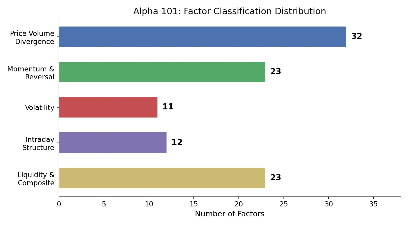
With the operators covered, we can look at the factors themselves. The 101 formulas may seem all over the place, but by economic logic, they fall into five categories.
Price-Volume Divergence (32 Factors)
Core thesis: price and volume should move in sync. When price rises on shrinking volume, the rally may lack conviction. When volume surges without much price movement, buyers and sellers disagree, and a directional breakout may be coming.
Price-volume divergence is one of the oldest ideas in technical analysis. Alpha 101 formalized it.
Alpha#3 is the cleanest example of this category:
$$\text{Alpha#3} = -1 \times \text{correlation}(\text{rank}(\text{open}),\ \text{rank}(\text{volume}),\ 10)$$Layer by layer:
rank(open): Rank all stocks by opening price on each day, normalize to 0–1rank(volume): Rank all stocks by volume on each day, normalize to 0–1correlation(..., 10): Pearson correlation of these two rank series over the past 10 days-1 *: Flip the sign
If a stock’s opening-price rank and volume rank have been moving together over the past 10 days (positive correlation), the factor gives a negative value (short signal). If they have been diverging (negative correlation), the factor gives a positive value (long signal).
Why is price-volume divergence a buy signal? One interpretation: when the opening price rises but volume does not follow, the move is not driven by retail chasing, so it may reflect slow fundamental repricing. When both price and volume surge together, the stock is more likely overheated in the short term.
Alpha#12 is more direct:
$$\text{Alpha#12} = \text{sign}(\text{delta}(\text{volume}, 1)) \times (-1 \times \text{delta}(\text{close}, 1))$$In plain terms: if today’s volume is higher than yesterday’s (sign(delta(volume, 1)) = +1), bet against today’s price direction (multiply by -1 * delta(close, 1)). If volume dropped, bet with today’s price direction.
The logic: a rally on heavy volume is likely to reverse; a decline on light volume is likely to bounce. Abnormal price-volume alignment signals a reversal.
This category has the most factors (32 out of 101), which suggests WorldQuant found price-volume relationships to provide the largest number of independent short-term signals.
# Alpha#3 computation example
# df_open and df_volume are DataFrames with rows=dates, columns=stocks
alpha3 = -1 * ts_corr(rank(df_open), rank(df_volume), 10)
Momentum and Reversal (23 Factors)
Core thesis: stocks tend to reverse over very short horizons (1–5 days) and persist over medium horizons (10–20 days).
Short-term reversal has a straightforward economic explanation: stocks that rallied hard today attract profit-taking tomorrow, pushing prices back down. Stocks that sold off heavily get bottom-fished, pushing prices back up. This is a stable phenomenon in liquid markets, driven by market makers and short-term traders.
Medium-term momentum has a different source: information diffusion takes time. When good news breaks, not everyone reacts simultaneously. Smart money buys first, and less-informed participants follow, creating a trend.
Alpha#9 is a conditional reversal factor:
$$\text{Alpha#9} = \begin{cases} \text{ts_rank}(\text{delta}(\text{close},1),\ 5) & \text{if } 0 < \text{ts_min}(\text{delta}(\text{close},1),\ 5) \\ \text{ts_rank}(\text{delta}(\text{close},1),\ 5) & \text{if } \text{ts_max}(\text{delta}(\text{close},1),\ 5) < 0 \\ -1 \times \text{delta}(\text{close},1) & \text{otherwise} \end{cases}$$The first two conditions check for a consistent trend: if every day in the past 5 was up (minimum change > 0), or every day was down (maximum change < 0), use ts_rank to gauge how the current move compares to recent history. Otherwise (mixed up-and-down days), use a simple reversal signal. The two trend branches have identical formulas, and that is not a typo: the paper applies the same momentum measure to both “consistently up” and “consistently down” regimes. The sign difference comes from delta(close,1) itself being positive or negative.
What stands out: it uses momentum logic (ts_rank) during trending markets but switches to reversal logic in choppy markets. A single layer of regime detection on top of a naive reversal factor.
Alpha#20 targets gap fills:
$$\text{Alpha#20} = -1 \times \text{rank}(\text{open} - \text{delay}(\text{high}, 1)) \times \text{rank}(\text{open} - \text{delay}(\text{close}, 1)) \times \text{rank}(\text{open} - \text{delay}(\text{low}, 1))$$All three terms measure where today’s open sits relative to yesterday’s candlestick. If today gapped up above yesterday’s high, close, and low, all three terms are positive, their product is positive, and the -1 makes the factor negative (short signal). The logic: large gap-ups tend to be overreactions that get partially filled during the day.
Volatility (11 Factors)
Core thesis: volatility mean-reverts. Periods of high volatility tend to subside; periods of low volatility tend to expand.
More precisely, volatility factors try to identify regime transitions. When a quiet stock suddenly makes a big move, it often signals new information arrival and the start of a trend. Conversely, after sustained high volatility, the market digests the information and volatility contracts.
Alpha#1 is a conditional volatility signal:
$$\text{Alpha#1} = \text{rank}\Big(\text{ts_argmax}\big(\text{signedpower}(\text{returns} < 0\ ?\ \text{stddev}(\text{returns}, 20)\ :\ \text{close},\ 2),\ 5\big)\Big) - 0.5$$Step by step: pick the signal source conditionally (volatility during declines, closing price during rallies), apply signedpower to amplify differences, use ts_argmax to find where the 5-day maximum sits in the window, then cross-sectionally rank and subtract 0.5 to center the factor around zero (positive = long, negative = short).
The underlying intuition: in a down market, focus on volatility, because extreme volatility during sell-offs signals peak panic, and peak panic tends to precede reversals. In an up market, focus on price levels.
The volatility category has only 11 factors, but the underlying logic connects directly to volatility trading strategies: volatility itself is a tradeable quantity.
Intraday Structure (12 Factors)
Core thesis: the relative positions of open, close, high, low, and VWAP within the daily bar encode information about intraday trader behavior.
How much did the stock gain from open to close (intraday return)? Where does the close sit within the day’s range (near the high or the low)? Is VWAP above or below close (were institutions trading above or below the final price)?
Alpha#101 has the simplest structure:
$$\text{Alpha#101} = \frac{\text{close} - \text{open}}{(\text{high} - \text{low}) + 0.001}$$Numerator is the intraday gain; denominator is the intraday range (plus 0.001 to avoid division by zero). The ratio measures what fraction of the day’s range was captured as directional return. A value near +1 means the stock opened at the low and closed at the high (unidirectional rally all day). A value near 0 means the close was about the same as the open despite intraday swings.
This is a classic technical indicator known as the “close location value.” Its predictive interpretation: stocks with strong unidirectional days tend to show (weak) continuation the next day. Stocks that churned all day with no net progress lack directional momentum.
Alpha#42 looks at VWAP vs. close:
$$\text{Alpha#42} = \frac{\text{rank}(\text{vwap} - \text{close})}{\text{rank}(\text{vwap} + \text{close})}$$When vwap - close > 0, the volume-weighted average transaction price exceeds the closing price, meaning “most trading happened at higher prices and the stock drifted down toward the close.” This is often a sign that institutions were distributing (selling) throughout the day. The factor treats this as a bearish signal.
Note that Alpha#42 uses no delay: all inputs are from the current day. The paper lists its holding period as approximately 0 days, making it a purely intraday signal. In T+1 markets like Chinese A-shares, this factor cannot be directly applied.
Liquidity and Composite (23 Factors)
Core thesis: changes in liquidity (volume, turnover) reflect institutional money flow.
Large institutional orders cannot be filled in a single trade. When a stock shows elevated volume for several consecutive days but little price movement, someone may be building a position in slices. A sudden volume drop may signal the accumulation is done or the market has shifted to wait-and-see.
Alpha#7 is a conditional liquidity signal:
$$\text{Alpha#7} = \begin{cases} -1 \times \text{ts_rank}(\text{abs}(\text{delta}(\text{close},7)),\ 60) \times \text{sign}(\text{delta}(\text{close},7)) & \text{if } \text{adv20} < \text{volume} \\ -1 & \text{otherwise} \end{cases}$$The condition: is today’s volume above the 20-day average? If yes (elevated volume), the factor uses the 7-day absolute price change, ranked within 60 days, multiplied by the direction, then flipped. If volume is below average (quiet day), it defaults to -1 (short signal).
The logic: on quiet days, go short, because low participation means weak support. On active days, assess the “magnitude” of the price move relative to recent history. Larger moves on high volume carry more meaning.
These factors tend to be complex, often nesting multiple operators and conditional branches. They blend volume, price, and volatility information into a single score. Parsing them one by one can be tedious, but the common thread is detecting where institutional-scale money is flowing.
Complete Alpha 101 Classification Reference
The table below assigns all 101 factors to five categories. The “Core Operators” column highlights the most important computation in each formula. “IndNeut” marks whether industry neutralization is required.
| # | Category | Core Operators | One-Line Logic | IndNeut | Series Part |
|---|---|---|---|---|---|
| 1 | Volatility | stddev, ts_argmax | Volatility extremes during down markets | No | Part 4 |
| 2 | Price-Vol | correlation, rank | Price-volume rank correlation + intraday move | No | Part 2 |
| 3 | Price-Vol | correlation, rank | Open-volume rank correlation | No | Part 2 |
| 4 | Momentum | ts_rank | Low-rank short signal | No | Part 3 |
| 5 | Intraday | rank, ts_rank, vwap | VWAP deviation rank change | No | Part 4 |
| 6 | Price-Vol | correlation | Direct open-volume correlation | No | Part 2 |
| 7 | Liquidity | adv, ts_rank, delta | Conditional volume-price momentum | No | Part 5 |
| 8 | Momentum | rank, delta, sum | Open change vs. return rank interaction | No | Part 3 |
| 9 | Momentum | delta, ts_min/max | Conditional reversal: trending vs. choppy | No | Part 3 |
| 10 | Momentum | delta, ts_min/max | Conditional momentum variant of #9 | No | Part 3 |
| 11 | Price-Vol | rank, correlation, vwap | VWAP/close/volume interaction | No | Part 2 |
| 12 | Price-Vol | sign, delta | Volume change direction × price change | No | Part 2 |
| 13 | Price-Vol | rank, covariance | Close-volume covariance rank | No | Part 2 |
| 14 | Price-Vol | correlation, returns | Open-return correlation | No | Part 2 |
| 15 | Price-Vol | correlation, rank | High-volume rank correlation | No | Part 2 |
| 16 | Price-Vol | covariance, rank | High-volume covariance rank | No | Part 2 |
| 17 | Price-Vol | rank, ts_rank, delta | Close rank vs. volume momentum rank | No | Part 2 |
| 18 | Volatility | correlation, stddev | Close-open correlation | No | Part 4 |
| 19 | Momentum | returns, delay | Conditional return reversal | No | Part 3 |
| 20 | Momentum | rank, open, delay | Gap fill reversal | No | Part 3 |
| 21 | Volatility | mean, stddev, close | Mean deviation + volume condition | No | Part 4 |
| 22 | Price-Vol | correlation, delta, stddev | High-volume correlation + price change | No | Part 2 |
| 23 | Momentum | sma, delta, high | High-price mean conditional reversal | No | Part 3 |
| 24 | Momentum | sma, delta, close | Close-price mean conditional reversal | No | Part 3 |
| 25 | Price-Vol | rank, returns, adv, vwap | Return × volume deviation × VWAP rank | No | Part 2 |
| 26 | Price-Vol | correlation, ts_rank | Time-series rank correlation + volume | No | Part 2 |
| 27 | Price-Vol | rank, correlation | Price-volume correlation rank quantile | No | Part 2 |
| 28 | Price-Vol | correlation, adv, rank | Volume vs. average volume correlation | No | Part 2 |
| 29 | Momentum | delta, ts_rank, returns | Close change rank trend | No | Part 3 |
| 30 | Momentum | delta, close, volume | Price-volume change sign interaction | No | Part 3 |
| 31 | Liquidity | rank, adv, correlation, decay_linear | Liquidity + decayed price-volume correlation | No | Part 5 |
| 32 | Price-Vol | scale, correlation | Mean deviation × decayed price-volume correlation | No | Part 2 |
| 33 | Momentum | rank, open/close | Open-close rank reversal | No | Part 3 |
| 34 | Volatility | rank, stddev, delta | Volatility rank + price reversal | No | Part 4 |
| 35 | Momentum | rank, returns, volume, ts_rank | Multi-factor composite reversal | No | Part 3 |
| 36 | Volatility | correlation, rank, adv | Multi-dimensional correlation rank | No | Part 4 |
| 37 | Momentum | correlation, rank, delay | Open rank autocorrelation | No | Part 3 |
| 38 | Momentum | rank, close, open | Close rank vs. intraday change | No | Part 3 |
| 39 | Momentum | rank, delta, decay_linear | Decayed momentum signal | No | Part 3 |
| 40 | Price-Vol | rank, stddev, correlation | High-price volatility × volume rank | No | Part 2 |
| 41 | Intraday | high, low, vwap | Intraday range vs. VWAP | No | Part 4 |
| 42 | Intraday | rank, vwap, close | VWAP-close deviation | No | Part 4 |
| 43 | Price-Vol | rank, adv, delta | Liquidity rank × price change | No | Part 2 |
| 44 | Price-Vol | correlation, rank | Low-volume rank correlation | No | Part 2 |
| 45 | Price-Vol | rank, delta, correlation, decay_linear | Close change rank × decayed price-vol corr | No | Part 2 |
| 46 | Momentum | delay, delta, close | Conditional price momentum | No | Part 3 |
| 47 | Intraday | rank, adv, high, close, vwap | Liquidity-weighted VWAP-close deviation | No | Part 4 |
| 48 | Liquidity | correlation, rank, delta | Industry-neutral price-volume corr | Yes | Part 5 |
| 49 | Momentum | delta, delay, close | Conditional price reversal | No | Part 3 |
| 50 | Price-Vol | correlation, rank, ts_rank | Price-volume rank time-series corr | No | Part 2 |
| 51 | Momentum | delta, delay, close | Conditional delayed reversal | No | Part 3 |
| 52 | Momentum | delta, ts_min, ts_rank | Price trough + volume rank | No | Part 3 |
| 53 | Momentum | delta, close, high, low | Intraday position change | No | Part 3 |
| 54 | Intraday | open, close, low | Intraday deviation structure | No | Part 4 |
| 55 | Price-Vol | correlation, rank | Intraday range vs. volume correlation | No | Part 2 |
| 56 | Momentum | rank, returns, cap | Market cap × return rank interaction | No | Part 3 |
| 57 | Volatility | decay_linear, rank, ts_argmin | Decayed trough position rank | No | Part 4 |
| 58 | Liquidity | correlation, rank, volume | Industry-neutral price-volume corr | Yes | Part 5 |
| 59 | Liquidity | correlation, rank, volume | Industry-neutral price-volume corr variant | Yes | Part 5 |
| 60 | Price-Vol | scale, correlation, rank | Price-vol corr × scaled intraday change | No | Part 2 |
| 61 | Liquidity | rank, vwap, adv | VWAP rank vs. average volume rank | No | Part 5 |
| 62 | Intraday | rank, vwap, correlation, adv | VWAP rank × price-volume corr | No | Part 4 |
| 63 | Liquidity | rank, vwap, delta, decay_linear, adv | Decayed liquidity signal | Yes | Part 5 |
| 64 | Intraday | rank, correlation, vwap, adv | VWAP-liquidity correlation rank | Yes | Part 4 |
| 65 | Intraday | rank, correlation, vwap, adv | VWAP rank correlation decay | Yes | Part 4 |
| 66 | Intraday | rank, decay_linear, vwap, delta | VWAP deviation decayed momentum | Yes | Part 4 |
| 67 | Liquidity | rank, correlation, high, adv | High-price vs. average volume corr rank | Yes | Part 5 |
| 68 | Intraday | rank, correlation, high, adv, close | High-volume corr × close rank | Yes | Part 4 |
| 69 | Liquidity | rank, ts_rank, delta, close, adv | Industry-neutral price momentum rank | Yes | Part 5 |
| 70 | Liquidity | rank, delta, close, vwap | Industry-neutral price-VWAP change | Yes | Part 5 |
| 71 | Liquidity | decay_linear, correlation, rank, close, adv | Multi-layer decayed liquidity signal | Yes | Part 5 |
| 72 | Liquidity | rank, correlation, vwap, adv, decay_linear | Decayed price-volume rank corr | Yes | Part 5 |
| 73 | Intraday | rank, decay_linear, vwap, delta, open | VWAP decay × open change | Yes | Part 4 |
| 74 | Price-Vol | rank, correlation, close, adv | Close vs. average volume corr rank | Yes | Part 2 |
| 75 | Liquidity | rank, correlation, vwap, volume | VWAP vs. volume rank correlation | No | Part 5 |
| 76 | Liquidity | rank, decay_linear, correlation, vwap | Decayed VWAP rank corr | Yes | Part 5 |
| 77 | Price-Vol | rank, decay_linear, delta, correlation | Decayed price change × price-vol corr | No | Part 2 |
| 78 | Price-Vol | rank, correlation, low, adv | Low vs. average volume corr rank | No | Part 2 |
| 79 | Liquidity | rank, delta, vwap, correlation, close | Industry-neutral VWAP change rank | Yes | Part 5 |
| 80 | Liquidity | rank, delta, close, correlation, adv | Industry-neutral change + price-vol corr | Yes | Part 5 |
| 81 | Price-Vol | rank, correlation, vwap, adv | VWAP vs. average volume rank corr | No | Part 2 |
| 82 | Liquidity | rank, delta, open, correlation, adv | Industry-neutral open change rank | Yes | Part 5 |
| 83 | Volatility | rank, delay, high, low | Lagged intraday range rank | No | Part 4 |
| 84 | Momentum | rank, vwap, close, signedpower | VWAP-close deviation powered | No | Part 3 |
| 85 | Price-Vol | rank, correlation, high, adv | High rank vs. avg volume corr | No | Part 2 |
| 86 | Volatility | rank, correlation, close, adv, delay | Lagged price-volume corr conditional | Yes | Part 4 |
| 87 | Liquidity | rank, decay_linear, delta, vwap, adv | Decayed VWAP momentum | Yes | Part 5 |
| 88 | Price-Vol | rank, decay_linear, correlation, open | Open rank decayed correlation | No | Part 2 |
| 89 | Liquidity | decay_linear, correlation, rank | Decayed correlation signal | No | Part 5 |
| 90 | Momentum | rank, correlation, close, adv | Close vs. avg volume rank corr reversal | No | Part 3 |
| 91 | Liquidity | rank, correlation, close, adv, decay_linear | Close-volume decayed corr | Yes | Part 5 |
| 92 | Price-Vol | rank, decay_linear, delta, correlation | Multi-dimensional decayed price-vol signal | No | Part 2 |
| 93 | Liquidity | rank, correlation, vwap, adv, decay_linear | Industry-neutral decayed VWAP corr | Yes | Part 5 |
| 94 | Volatility | rank, correlation, adv | Volume rank and low-price signal | No | Part 4 |
| 95 | Price-Vol | rank, correlation, high, adv | High rank vs. avg volume corr | No | Part 2 |
| 96 | Volatility | decay_linear, rank, ts_argmax, correlation | Decayed extremum position × price-vol corr | No | Part 4 |
| 97 | Liquidity | rank, decay_linear, delta, correlation, adv | Industry-neutral decayed liquidity | Yes | Part 5 |
| 98 | Volatility | rank, decay_linear, correlation, vwap, adv | Decayed VWAP corr rank | No | Part 4 |
| 99 | Price-Vol | rank, correlation, high, volume | High vs. volume rank correlation | No | Part 2 |
| 100 | Liquidity | rank, stddev, correlation, adv | Volatility-liquidity corr rank | Yes | Part 5 |
| 101 | Intraday | close, open, high, low | Intraday return as fraction of range | No | Part 4 |
Practical Tips
The decimal parameters are machine-optimized noise. Alpha#4 has a window of 9.99922. Alpha#35 includes 2.21. These numbers came from automated optimization, not human judgment. They are almost certainly overfit to the in-sample period. Rounding to the nearest integer (10, 2) likely gives similar out-of-sample performance.
26 factors require industry classification data. Factors marked “IndNeut” in the table above use IndNeutralize, which requires an industry label for every stock. For US equities, use GICS or SIC codes. For Chinese A-shares, use Shenwan (申万) industry classification. If you don’t have industry data, start with the other 75 factors.
Some factors are purely intraday signals. Alpha#42 and #54, for example, use no delay and rely entirely on same-day OHLCV data. The paper lists their holding periods as approximately 0 days. In T+1 markets (Chinese A-shares), these cannot be executed directly. You can lag the signals by one day as next-day selection factors, but expect degraded performance.
A single factor is not a strategy. The paper was published in 2016, a decade ago. Any individual factor suffers alpha decay after publication as more people trade the same signal. But the classification logic does not expire: price-volume divergence, momentum reversal, and volatility mean-reversion are economic regularities that do not disappear because a paper was published.
These factors were designed for US large-caps. The 101 alphas were developed on a universe of roughly 1,000 US large-cap equities, with dollar-neutral and market-cap-weighted constraints. Applying them directly to Chinese A-share small-caps or other markets can produce very different results. A-share specifics like T+1 settlement, daily price limits, and a higher retail participation rate all affect factor behavior, especially for reversal and intraday factors. Always run local backtests before trusting any cross-market transfer.
The correct use of Alpha 101 is as building blocks. Combine factors into a multi-factor model. The average pairwise correlation of 15.9% means the factors capture different dimensions of information and diversify well in combination. For evaluating the resulting portfolio, see the quant metrics guide covering Sharpe ratio, maximum drawdown, and related measures.
Series Roadmap
This is Part 1 of the Alpha 101 series. The next four articles go category by category:
- Part 2: Price-Volume Divergence (32 factors). The many ways to measure price-volume relationships
- Part 3: Momentum and Reversal (23 factors). When to follow the trend and when to bet on mean reversion
- Part 4: Volatility and Intraday Structure (23 factors). Volatility mean-reversion + OHLCV intraday information
- Part 5: Liquidity, Composite Factors, and Multi-Factor Portfolios (23 factors). From single factors to portfolio construction
If you are not yet familiar with standard portfolio evaluation metrics, start with the quant metrics guide for Sharpe ratio, maximum drawdown, and more. The volatility factors connect directly to ideas in volatility trading strategies, which may be worth reading in parallel.